Lampiran 1. Gambar Nata
(a)
(b)
(c)
Gambar 11.
Nata de Apple
Hasil Uji Pendahuluan dalam Plastik
Box
dengan Berbagai
Konsentrasi Starter (a) 10%, (b) 20%, dan (c) 30%
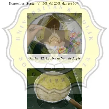
Gambar 12. Lembaran
Nata de Apple
Gambar 13. Perebusan
Nata de apple
Lampiran 3.
Worksheet
Uji
Rating
Hedonik Nata
WORKSHEET
UJI RATING HEDONIK
Tanggal
: 1 Febuari 2011
Jenis sample : Nata
Identifikasi
Kode
Nata de Apple sari murni ZA
A
Nata de Apple sari murni Yeast
B
Nata de Apple sari ampas ZA
C
Nata de Apple sari ampas Yeast
D
Nata de Coco
E
Kode kombinasi urutan penyajian
ABCDE = 1
ACDEB = 6
BCDAE = 2
BECAD = 7
CDABE = 3
DEBAC = 8
DABCE = 4
ECABD = 9
EABCD = 5
BCDEA = 10
Rekap kode sampel
Lampiran 4.
Scoresheet
Uji
Rating
Hedonik Nata
UJI RATING HEDONIK
Nama
:
Tanggal
:
Produk
: Nata
Kriteria
:
Warna
Instruksi :
Di hadapan Anda terdapat 5 sampel produk nata.
Amatilah masing-masing sampel. Berilah skor (1) untuk sampel dengan warna yang paling
tidak disukai hingga skor (7) untuk sampel dengan warna yang paling disukai. Pemberian
skor untuk tiap-tiap sampel boleh mengalami pengulangan.
---
---
---
---
---
---
---
---
---
---
UJI RATING HEDONIK
Nama
:
Tanggal
:
Produk
: Nata
Kriteria
:
Kekenyalan
Instruksi :
Di hadapan Anda terdapat 5 sampel produk nata.
Ambil masing-masing sampel dan gigit sampel dengan gigi Anda. Berilah skor (1) untuk
sampel dengan tingkat kekenyalan yang paling tidak disukai hingga skor (7) untuk sampel
tingkat kekenyalan yang paling disukai. Pemberian skor untuk tiap-tiap sampel boleh
mengalami pengulangan.
UJI RATING HEDONIK
Nama
:
Tanggal
:
Produk
: Nata
Kriteria
: Overall
Instruksi :
Di hadapan Anda terdapat 5 sampel produk nata.
Amatilah masing-masing sampel. Berilah skor (1) untuk sampel yang paling tidak disukai
hingga skor (7) untuk sampel yang paling disukai. Pemberian skor untuk tiap-tiap sampel
boleh mengalami pengulangan.
Lampiran 5. SPSS Uji Normalitas Karakteristik Fisik dan Kimia Berbagai
Perlakuan
Nata de Apple
Tests of Normality
perlakuan
Kolmogorov-Smirnov(a) Shapiro-Wilk
Statistic df Sig. Statistic df Sig. Tebal 1.00 .267 6 .200(*) .936 6 .624
* This is a lower bound of the true significance. a Lilliefors Significance Correction
Lampiran 6. SPSS Uji Beda Karakteristik Fisik dan Kimia Berbagai Perlakuan
Nata
de Apple
ANOVA
Sum of
Squares df Mean Square F Sig. tebal Between Groups .140 3 .047 15.313 .000
Within Groups .061 20 .003
Total .200 23
kekerasan Between Groups 1155.149 3 385.050 8.111 .001 Within Groups 949.436 20 47.472
Total 2104.585 23
kekenyalan Between Groups .375 3 .125 12.958 .000 Within Groups .193 20 .010
Total .568 23
pH_sebelum Between Groups .386 3 .129 114.189 .000 Within Groups .023 20 .001
Total .409 23
pH_sesudah Between Groups .410 3 .137 64.289 .000 Within Groups .043 20 .002
Total .453 23
gula_sebelum Between Groups 192.155 3 64.052 124.816 .000 Within Groups 10.263 20 .513
Total 202.418 23
gula_sesudah Between Groups 185.151 3 61.717 58.421 .000 Within Groups 21.128 20 1.056
Total 206.280 23
serat_kasar Between Groups .686 3 .229 12.095 .000 Within Groups .378 20 .019
ANOVA
Sum of
Squares df Mean Square F Sig. murni_za Between Groups .108 1 .108 94.174 .000
Within Groups .012 10 .001
Total .120 11
murni_yeast Between Groups .068 1 .068 60.994 .000 Within Groups .011 10 .001
Total .079 11
ampas_za Between Groups .118 1 .118 65.258 .000 Within Groups .018 10 .002
Total .136 11
ampas_yeast Between Groups .120 1 .120 49.046 .000 Within Groups .024 10 .002
Total .144 11
ANOVA
Sum of
Squares df Mean Square F Sig. murni_za Between Groups 1.203 1 1.203 3.989 .074
Within Groups 3.017 10 .302
Total 4.220 11
murni_yeast Between Groups 18.750 1 18.750 12.266 .006 Within Groups 15.287 10 1.529
Total 34.037 11
ampas_za Between Groups 2.803 1 2.803 5.555 .040 Within Groups 5.047 10 .505
Total 7.850 11
ampas_yeast Between Groups 15.188 1 15.188 18.886 .001 Within Groups 8.042 10 .804
tebal
Duncan
perlakuan
N Subset for alpha = .05
1 2 1
1.00 6 .8950
3.00 6 1.0450
2.00 6 1.0500
4.00 6 1.0983
Sig. 1.000 .128 Means for groups in homogeneous subsets are displayed. a Uses Harmonic Mean Sample Size = 6.000.
kekerasan
Duncan
perlakuan
N Subset for alpha = .05
1 2 3 1
1.00 6 25.6206
3.00 6 32.9971 32.9971 4.00 6 39.8779 39.8779
2.00 6 43.8378
Sig. .078 .099 .331 Means for groups in homogeneous subsets are displayed.
a Uses Harmonic Mean Sample Size = 6.000.
kekenyalan
Duncan
perlakuan
N Subset for alpha = .05
1 2 3 1
2.00 6 .0690
4.00 6 .1946
3.00 6 .3648
1.00 6 .3665
Sig. 1.000 1.000 .976 Means for groups in homogeneous subsets are displayed.
pH_sebelum
Duncan
perlakuan
N Subset for alpha = .05
1 2 3 1
1.00 6 3.2650
3.00 6 3.3033
2.00 6 3.4567
4.00 6 3.5833
Sig. .062 1.000 1.000 Means for groups in homogeneous subsets are displayed.
a Uses Harmonic Mean Sample Size = 6.000.
pH_sesudah
Duncan
perlakuan
N Subset for alpha = .05
1 2 3 1
1.00 6 3.0750
3.00 6 3.1050
2.00 6 3.3067
4.00 6 3.3833
Sig. .273 1.000 1.000 Means for groups in homogeneous subsets are displayed.
a Uses Harmonic Mean Sample Size = 6.000.
gula_sebelum
Duncan
perlakuan
N Subset for alpha = .05
1 2 3 1
3.00 6 11.1333
4.00 6 11.4167
1.00 6 15.7167
2.00 6 17.7667
Sig. .501 1.000 1.000 Means for groups in homogeneous subsets are displayed.
gula_sesudah
Duncan
perlakuan
N Subset for alpha = .05
1 2 1
4.00 6 9.1667
3.00 6 10.1667 1.00 6 15.0833 2.00 6 15.2667 Sig. .107 .761 Means for groups in homogeneous subsets are displayed. a Uses Harmonic Mean Sample Size = 6.000.
serat_kasar
Duncan
perlakuan
N Subset for alpha = .05
1 2 1
1.00 6 1.1083
3.00 6 1.4400
2.00 6 1.4550
4.00 6 1.5583
Sig. 1.000 .173 Means for groups in homogeneous subsets are displayed. a Uses Harmonic Mean Sample Size = 6.000.
Lampiran 7. SPSS Uji Beda pada Sensori
Nata de Apple
Kruskal-Wallis Test
Test Statistics(a,b)
warna kekenyalan overall Chi-Square 71.530 46.030 68.545
df 4 4 4
Asymp. Sig. .000 .000 .000 a Kruskal Wallis Test
Mann-Whitney Test
1 vs 2
Test Statistics(a)
warna kekenyalan overall Mann-Whitney U 288.500 219.000 133.500 Wilcoxon W 753.500 684.000 598.500 Z -2.473 -3.512 -4.830 Asymp. Sig. (2-tailed) .013 .000 .000 a Grouping Variable: perlakuan
2 vs 3
Test Statistics(a)
warna kekenyalan overall Mann-Whitney U 443.000 394.500 450.000 Wilcoxon W 908.000 859.500 915.000
Z -.107 -.843 .000
Asymp. Sig. (2-tailed) .915 .399 1.000 a Grouping Variable: perlakuan
2 vs 4
Test Statistics(a)
3 vs 4
Test Statistics(a)
warna kekenyalan overall Mann-Whitney U 152.500 271.500 226.500 Wilcoxon W 617.500 736.500 691.500 Z -4.514 -2.711 -3.442 Asymp. Sig. (2-tailed) .000 .007 .001 a Grouping Variable: perlakuan
3 vs 5
Test Statistics(a)
kekenyalan overall Mann-Whitney U 325.500 201.000 Wilcoxon W 790.500 666.000
Z -1.903 -3.839
Asymp. Sig. (2-tailed) .057 .000 a Grouping Variable: perlakuan
4 vs 5
Test Statistics(a)
warna kekenyalan overall Mann-Whitney U 396.000 438.000 427.500 Wilcoxon W 861.000 903.000 892.500
Z -.846 -.184 -.362