Still Image and Video Compression with MATLAB

(1)

(2)

(3)

(4)

STILL IMAGE AND

VIDEO COMPRESSION

WITH MATLAB

K. S. Thyagarajan

(5)

No part of this publication may be reproduced, stored in a retrieval system, or transmitted in any form or by any means, electronic, mechanical, photocopying, recording, scanning, or otherwise, except as permitted under Section 107 or 108 of the 1976 United States Copyright Act, without either the prior written permission of the Publisher, or authorization through payment of the appropriate per-copy fee to the Copyright Clearance Center, Inc., 222 Rosewood Drive, Danvers, MA 01923, 978-750-8400, fax 978-750-4470, or on the web at www.copyright.com. Requests to the Publisher for permission should be addressed to the Permissions Department, John Wiley & Sons, Inc., 111 River Street, Hoboken, NJ 07030, 201-748-6011, fax 201-748-6008, or online at http://www.wiley.com/go/permission. Limit of Liability/Disclaimer of Warranty: While the publisher and author have used their best efforts in preparing this book, they make no representations or warranties with respect to the accuracy or completeness of the contents of this book and specifically disclaim any implied warranties of merchantability or fitness for a particular purpose. No warranty may be created or extended by sales representatives or written sales materials. The advice and strategies contained herein may not be suitable for your situation. You should consult with a professional where appropriate. Neither the publisher nor author shall be liable for any loss of profit or any other commercial damages, including but not limited to special, incidental, consequential, or other damages.

For general information on our other products and services or for technical support, please contact our Customer Care Department within the United States at 877-762-2974, outside the United States at 317-572-3993 or fax 317- 572-4002.

Wiley also publishes its books in a variety of electronic formats. Some content that appears in print may not be available in electronic formats. For more information about Wiley products, visit our web site at www.wiley.com.

Library of Congress Cataloging-in-Publication Data:

Thyagarajan, K. S.

Still image and video compression with MATLAB / K.S. Thyagarajan. p. cm.

ISBN 978-0-470-48416-6 (hardback)

1. Image compression. 2. Video compression. 3. MATLAB. I. Title. TA1638.T48 2010

006.6′_96–dc22

2010013922 Printed in Singapore

(6)

To my wife Vasu,

(7)

(8)

PREFACE

The term “video compression” is now a common household name. The field of still image and video compression has matured to the point that it is possible to watch movies on a laptop computer. Such is the rapidity at which technology in various fields has advanced and is advancing. However, this creates a need for some to obtain at least a simple understanding behind all this. This book attempts to do just that, to explain the theory behind still image and video compression methods in an easily understandable manner. The readers are expected to have an introductory knowledge in college-level mathematics and systems theory.

The properties of a still image are similar to those of a video, yet different. A still image is a spatial distribution of light intensity, while a video consists of a sequence of such still images. Thus, a video has an additional dimension—the temporal di-mension. These properties are exploited in several different ways to achieve data compression. A particular image compression method depends on how the image properties are manipulated.

Due to the availability of efficient, high-speed central processing units (CPUs), many Internet-based applications offer software solutions to displaying video in real time. However, decompressing and displaying high-resolution video in real time, such as high-definition television (HDTV), requires special hardware processors. Several such real-time video processors are currently available off the shelf. One can appreciate the availability of a variety of platforms that can decompress and dis-play video in real time from the data received from a single source. This is possible because of the existence of video compression standards such as Moving Picture Experts Group (MPEG).

This book first describes the methodologies behind still image and video com-pression in a manner that is easy to comprehend and then describes the most popular standards such as Joint Photographic Experts Group (JPEG), MPEG, and advanced video coding. In explaining the basics of image compression, care has been taken to keep the mathematical derivations to a minimum so that students as well as prac-ticing professionals can follow the theme easily. It is very important to use simpler mathematical notations so that the reader would not be lost in a maze. Therefore, a sincere attempt has been made to enable the reader to easily follow the steps in the book without losing sight of the goal. At the end of each chapter, problems are offered so that the readers can extend their knowledge further by solving them.

(13)

xii PREFACE

Whether one is a student, a professional, or an academician, it is not enough to just follow the mathematical derivations. For longer retention of the concepts learnt, one must have hands-on experience. The second goal of this book, therefore, is to work out real-world examples through computer software. Although many computer programming languages such as C, C++, Java, and so on are available, I chose MAT-LAB as the tool to develop the codes in this book. Using MATMAT-LAB to develop source code in order to solve a compression problem is very simple, yet it covers all grounds. Readers do not have to be experts in writing cleaver codes. MATLAB has many built-in functions especially for image and video processing that one can employ wherever needed. Another advantage of MATLAB is that it is similar to the C language. Furthermore, MATLAB SIMULINK is a very useful tool for actual simulation of different video compression algorithms, including JPEG and MPEG.

The organization of the book is as follows.

Chapter 1 makes an argument in favor of compression and goes on to introduce the terminologies of still image and video compression.

However, one cannot process an image or a video before acquiring data that is dealt within Chapter 2. Chapter 2 explains the image sampling theory, which relates pixel density to the power to resolve the smallest detail in an image. It further elu-cidates the design of uniform and nonuniform quantizers used in image acquisition devices. The topic of sampling using nonrectangular grids—such as hexagonal sam-pling grids—is not found in most textbooks on image or video compression. The hexagonal sampling grids are used in machine vision and biomedicine. Chapter 2 also briefly demonstrates such a sampling technique with an example using MAT-LAB code to convert an image from rectangular to a hexagonal grid and vice versa.

Image transforms such as the discrete cosine transform and wavelet transform are the compression vehicles used in JPEG and MPEG standards. Therefore, uni-tary image transforms are introduced in Chapter 3. Chapter 3 illustrates the useful properties of such unitary transforms and explains their compression potential using several examples. Many of the examples presented also include analytical solutions. The theory of wavelet transform has matured to such an extent that it is deemed necessary to devote a complete chapter to it. Thus, Chapter 4 describes the essentials of discrete wavelet transform (DWT), its type such as orthogonal and biorthogonal transforms, efficient implementation of the DWT via subband coding, and so on. The idea of decomposing an image into a multilevel DWT using octave-band splitting is developed in Chapter 4 along with examples using real images.

(14)

PREFACE xiii The first type of lossy compression, namely, the predictive coding, is introduced in Chapter 6. It explains both one-dimensional and two-dimensional predictive cod-ing methods followed by the calculation of the predictor performance gain with ex-amples. This chapter also deals with the design of both nonadaptive and adaptive differential pulse code modulations, again with several examples.

Transform coding technique and its performance are next discussed in Chapter 7. It also explains the compression part of the JPEG standard with an example using MATLAB.

The wavelet domain image compression topic is treated extensively in Chapter 8. Examples are provided to show the effectiveness of both orthogonal and biorthogonal DWTs in compressing an image. The chapter also discusses the JPEG2000 standard, which is based on wavelet transform.

Moving on to video, Chapter 9 introduces the philosophy behind compressing video sequences. The idea of motion estimation and compensation is explained along with subpixel accurate motion estimation and compensation. Efficient techniques such as hierarchical and pyramidal search procedures to estimate block motion are introduced along with MATLAB codes to implement them. Chapter 9 also introduces stereo image compression. The two images of a stereo image pair are similar yet dif-ferent. By using motion compensated prediction, the correlation between the stereo image pair is reduced and hence compression achieved. A MATLAB-based example illustrates this idea clearly.

The concluding chapter, Chapter 10, describes the video compression part of the MPEG-1, -2, -4, and H.264 standards. It also includes examples using MATLAB codes to illustrate the standards’ compression mechanism. Each chapter includes problems of increasing difficulty to help the students grasp the ideas discussed.

I thank Dr. Kesh Bakhru and Mr. Steve Morley for reviewing the initial book proposal and giving me continued support. My special thanks to Dr. Vinay Sathe of Multirate Systems for reviewing the manuscript and providing me with valuable comments and suggestions. I also thank Mr. Arjun Jain of Micro USA, Inc., for pro-viding me encouragement in writing this book. I wish to acknowledge the generous and continued support provided by The MathWorks in the form of MATLAB soft-ware. This book would not have materialized but for my wife Vasu, who is solely responsible for motivating me and persuading me to write this book. My heart-felt gratitude goes to her for patiently being there during the whole period of writing this book. She is truly the inspiration behind this work.

K. S. Thyagarajan

(15)

1

INTRODUCTION

This book is all about image and video compression. Chapter 1 simply introduces the overall ideas behind data compression by way of pictorial and graphical examples to motivate the readers. Detailed discussions on various compression schemes appear in subsequent chapters. One of the goals of this book is to present the basic principles behind image and video compression in a clear and concise manner and develop the necessary mathematical equations for a better understanding of the ideas. A further goal is to introduce the popular video compression standards such as Joint Photo-graphic Experts Group (JPEG) and Moving Picture Experts Group (MPEG) and ex-plain the compression tools used by these standards. Discussions on semantics and data transportation aspects of the standards will be kept to a minimum. Although the readers are expected to have an introductory knowledge in college-level mathematics and systems theory, clear explanations of the mathematical equations will be given where necessary for easy understanding. At the end of each chapter, problems are given in an increasing order of difficulty to make the understanding firm and lasting. In order for the readers of this book to benefit further, MATLAB codes for sev-eral examples are included. To run the M-files on your computers, you should in-stall MATLAB software. Although there are other software tools such as C++and Python to use, MATLAB appears to be more readily usable because it has a lot of built-in functions in various areas such as signal processing, image and video pro-cessing, wavelet transform, and so on, as well as simulation tools such as MATLAB Simulink. Moreover, the main purpose of this book is to motivate the readers to learn and get hands on experience in video compression techniques with easy-to-use software tools, which does not require a whole lot of programming skills. In the

(16)

2 INTRODUCTION

remainder of the chapter, we will briefly describe various compression techniques with some examples.

1.1 WHAT IS SOURCE CODING?

Images and videos are moved around the World Wide Web by millions of users al-most in a nonstop fashion, and then, there is television (TV) transmission round the clock. Analog TV has been phased out since February 2009 and digital TV has taken over. Now we have the cell phone era. As the proverba picture is worth a thousand wordsgoes, the transmission of these visual media in digital form alone will require far more bandwidth than what is available for the Internet, TV, or wireless networks. Therefore, one must find ways to format the visual media data in such a way that it can be transmitted over the bandwidth-limited TV, Internet, and wireless channels in real time. This process of reducing the image and video data so that it fits into the available limited bandwidth or storage space is termeddata compression. It is also calledsource codingin the communications field. When compressed audio/video data is actually transmitted through a transmission channel, extra bits are added to it to counter the effect of noise in the channel so that errors in the received data, if present, could be detected and/or corrected. This process of adding additional data bits to the compressed data stream before transmission is calledchannel coding. Ob-serve that the effect of reducing the original source data in source coding is offset to a small extent by the channel coding, which adds data rather than reducing it. How-ever, the added bits by the channel coder are very small compared with the amount of data removed by source coding. Thus, there is a clear advantage of compressing data.

We illustrate the processes of compressing and transmitting or storing a video source to a destination in Figure 1.1. The source of raw video may come from a video camera or from a previously stored video data. The source encoder compresses the raw data to a desired amount, which depends on the type of compression scheme chosen. There are essentially two categories of compression—losslessandlossy. In a lossless compression scheme, the original image or video data can be recovered exactly. In a lossy compression, there is always a loss of some information about the

Source decoder Still camera

Video camera

Disk

Source encoder

Entropy encoder

To transmission or storage

From transmission or storage

Entropy decoder

Disk

(17)

1.2 WHY IS COMPRESSION NECESSARY? 3 original data and so the recovered image or video data suffers from some form of dis-tortion, which may or may not be noticeable depending on the type of compression used. After source encoding, the quantized data is encoded losslessly for transmis-sion or storage. If the compressed data is to be transmitted, then channel encoder is used to add redundant or extra data bits and fed to the digital modulator. The digital modulator converts the input data into an RF signal suitable for transmission through a communications channel.

The communications receiver performs the operations of demodulation and chan-nel decoding. The chanchan-nel decoded data is fed to the entropy decoder followed by source decoder and is finally delivered to the sink or stored. If no transmission is used, then the stored compressed data is entropy decoded followed by source decod-ing as shown on the right-hand side of Figure 1.1.

1.2 WHY IS COMPRESSION NECESSARY?

An image or still image to be precise is represented in a computer as an array of numbers, integers to be more specific. An image stored in a computer is called a digital image. However, we will use the term image to mean a digital image. The image array is usually two dimensional (2D) if it is black and white (BW) and three dimensional (3D) if it is a color image. Each number in the array represents an in-tensity value at a particular location in the image and is called a picture element or pixel, for short. The pixel values are usually positive integers and can range between 0 and 255. This means that each pixel of a BW image occupies 1 byte in a computer memory. In other words, we say that the image has a grayscale resolution of 8 bits per pixel (bpp). On the other hand, a color image has a triplet of values for each pixel: one each for the red, green, and blue primary colors. Hence, it will need 3 bytes of storage space for each pixel. The captured images are rectangular in shape. The ratio of width to height of an image is called the aspect ratio. In standard-definition tele-vision (SDTV) the aspect ratio is 4:3, while it is 16:9 in a high-definition teletele-vision (HDTV). The two aspect ratios are illustrated in Figure 1.2, where Figure 1.2a cor-responds to an aspect ratio of 4:3 while Figure 1.2b corcor-responds to the same picture with an aspect ratio of 16:9. In both pictures, the height in inches remains the same,

2"

2.67" 3.56"

(a) (b)

2"

(18)

4 INTRODUCTION

which means that the number of rows remains the same. So, if an image has 480 rows, then the number of pixels in each row will be 480×4/3=640 for an aspect ratio of 4:3. For HDTV, there are 1080 rows and so the number of pixels in each row will be 1080×16/9=1920. Thus, a single SD color image with 24 bpp will require 640×480×3=921,600 bytes of memory space, while an HD color image with the same pixel depth will require 1920×1080×3=6,220,800 bytes. A video source may produce 30 or more frames per second, in which case the raw data rate will be 221,184,000 bits per second for SDTV and 1,492,992,000 bits per second for HDTV. If this raw data has to be transmitted in real time through an ideal communi-cations channel, which will require 1 Hz of bandwidth for every 2 bits of data, then the required bandwidth will be 110,592,000 Hz for SDTV and 746,496,000 Hz for HDTV. There are no such practical channels in existence that will allow for such a huge transmission bandwidth. Note that dedicated channels such as HDMI capable of transferring uncompressed data at this high rate over a short distance do exist, but we are only referring to long-distance transmission here. It is very clear that efficient data compression schemes are required to bring down the huge raw video data rates to manageable values so that practical communications channels may be employed to carry the data to the desired destinations in real time.

1.3 IMAGE AND VIDEO COMPRESSION TECHNIQUES

1.3.1 Still Image Compression

(19)

1.3 IMAGE AND VIDEO COMPRESSION TECHNIQUES 5

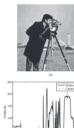
Figure 1.3 Original cameraman picture.

Having clarified the terms data compression and bandwidth compression, let us look into some basic data compression techniques known to us. Henceforth, we will use the terms compression and data compression interchangeably. All image and video sources have redundancies. In a still image, each pixel in a row may have a value very nearly equal to a neighboring pixel value. As an example, consider the cameraman picture shown in Figure 1.3. Figure 1.4 shows the profile (top figure)

0 50 100 150 200 250 300

0 100 200 300

Pixel number

Amplitude

Row 164

0 20 40 60 80 100 120 140

0.2 0.4 0.6 0.8 1

Pixel displacement

Nor

maliz

e

d corr

.

(20)

6 INTRODUCTION

and the corresponding correlation (bottom figure) of the cameraman picture along row 164. The MATLAB M-file for generating Figure 1.4 is listed below. Observe that the pixel values are very nearly the same over a large number of neighboring pixels and so is the pixel correlation. In other words, pixels in a row have a high cor-relation. Similarly, pixels may also have a high correlation along the columns. Thus, pixel redundancies translate to pixel correlation. The basic principle behind image data compression is todecorrelatethe pixels and encode the resulting decorrelated image for transmission or storage. A specific compression scheme will depend on the method by which the pixel correlations are removed.

Figure1 4.m

% Plots the image intensity profile and pixel correlation % along a specified row.

clear close all

I = imread(’cameraman.tif’);

figure,imshow(I),title(’Input image’) %

Row = 164; % row number of image profile x = double(I(Row,:));

Col = size(I,2); %

MaxN = 128; % number of correlation points to calculate Cor = zeros(1,MaxN); % array to store correlation values for k = 1:MaxN

l = length(k:Col);

Cor(k) = sum(x(k:Col) .* x(1:Col-k+1))/l; end

MaxCor = max(Cor); Cor = Cor/MaxCor;

figure,subplot(2,1,1),plot(1:Col,x,’k’,’LineWidth’,2) xlabel(’Pixel number’), ylabel(’Amplitude’)

legend([’Row’ ’ ’ num2str(Row)],0)

subplot(2,1,2),plot(0:MaxN-1,Cor,’k’,’LineWidth’,2) xlabel(’Pixel displacement’), ylabel(’Normalized corr.’)

(21)

1.3 IMAGE AND VIDEO COMPRESSION TECHNIQUES 7 Further, the residual image has a probability density function, which is a double-sided exponential function. These give rise to compression.

The quantizer is fixed no matter how the decorrelated pixel values are. A variation on the theme is to use quantizers that adapt to changing input statistics, and therefore, the corresponding DPCM is called an adaptive DPCM. DPCM is very simple to implement, but the compression achievable is about 4:1. Due to limited bit width of the quantizer for the residual image, edges are not preserved well in the DPCM. It also exhibits occasional streaks across the image when channel error occurs. We will discuss DPCM in detail in a later chapter.

(22)

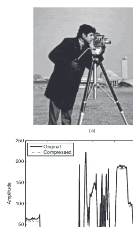
8 INTRODUCTION

(a)

(b)

0 50 100 150 200 250 300 0

50 100 150 200 250

Pixel number

Amplitude

Original Compressed

(23)

% Figure1 5.m

% Example to show blockiness in DCT compression % Quantizes and dequantizes an intensity image using % 8x8 DCT and JPEG quantization matrix

close all clear

figure,imshow(I), title(’Original Image’) %

fun = @dct2; % 2D DCT function N = 8; % block size of 2D DCT

T = blkproc(I,[N N],fun); % compute 2D DCT of image using NxN blocks %

Scale = 4.0; % increasing Scale quntizes DCT coefficients heavily % JPEG default quantization matrix

jpgQMat = [16 11 10 16 24 40 51 61;

12 12 14 19 26 58 60 55;

14 13 16 24 40 57 69 56;

14 17 22 29 51 87 80 62;

18 22 37 56 68 109 103 77; 24 35 55 64 81 194 113 92; 49 64 78 87 103 121 120 101; 72 92 95 98 121 100 103 99];

Qstep = jpgQMat * Scale; % quantization step size % Quantize and dequantize the coefficients for k = 1:N:size(I,1)

for l = 1:N:size(I,2)

T1(k:k+N-1,l:l+N-1) = round(T(k:k+N-1,l:l+N-1)./ Qstep).*Qstep; end

end

% do inverse 2D DCT fun = @idct2;

y = blkproc(T1,[N N],fun); y = uint8(round(y));

figure,imshow(y), title(’DCT compressed Image’) % Plot image profiles before and after compression ProfRow = 164;

figure,plot(1:size(I,2),I(ProfRow,:),’k’,’LineWidth’,2) hold on

plot(1:size(I,2),y(ProfRow,:),’-.k’,’LineWidth’,1) title([’Intensity profile of row ’ num2str(ProfRow)]) xlabel(’Pixel number’), ylabel(’Amplitude’)

%legend([’Row’ ’ ’ num2str(ProfRow)],0) legend(’Original’,’Compressed’,0)

(24)

10 INTRODUCTION

Figure 1.6 A two-level 2D DWT of cameraman image.

(25)

(a)

(b)

0 50 100 150 200 250 300 0

50 100 150 200 250

Pixel number

Amplitude

Original Compressed

(26)

12 INTRODUCTION

% Figure1 6.m

% 2D Discrete Wavelet Transform (DWT)

% Computes multi-level 2D DWT of an intensity image close all

clear

figure,imshow(I), title(’Original Image’) L = 2; % number of levels in DWT

[W,B] = wavedec2(I,L,’db2’); % do a 2-level DWT using db2 wavelet % declare level-1 subimages

w11 = zeros(B(3,1),B(3,1)); w12 = zeros(B(3,1),B(3,1)); w13 = zeros(B(3,1),B(3,1)); % declare level-2 subimages w21 = zeros(B(1,1),B(1,1)); w22 = zeros(B(1,1),B(1,1)); w23 = zeros(B(1,1),B(1,1)); w24 = zeros(B(1,1),B(1,1));

% extract level-1 2D DWT coefficients offSet11 = 4*B(1,1)*B(1,2);

% extract level-2 2D DWT coefficients offSet22 = B(1,1)*B(1,2);

% declare output array y to store all the DWT coefficients %y = zeros(261,261);

figure,imshow(y,[]),title([num2str(L) ’-level 2D DWT’])

% Figure1 7.m

(27)

% quantize only the approximation coefficients Qstep = 16; title([’Profile of row ’ num2str(ProfRow)]) xlabel(’Pixel number’), ylabel(’Amplitude’) %legend([’Row’ ’ ’ num2str(ProfRow)],0) legend(’Original’,’Compressed’,0)

1.3.2 Video Compression

(28)

14 INTRODUCTION

(a)

(c)

(e)

(d)

0 1000 2000 3000 4000 5000 6000 7000 8000

Pixel Value

Pixel Count

0 0.1 0.2 0.3 0.4 0.5 0.6 0.7 0.8 0.9 1 0 500 1000 1500

Pixel Value

Pixel Count

Pixel Value

0 50 100 150 200 250

(b)

(f)

(g)

(29)

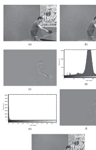
1.3 IMAGE AND VIDEO COMPRESSION TECHNIQUES 15 in Figure 1.8c. The differential frame has a small amount of details corresponding to the movements of the hand and the racket. Note that stationary objects do not appear in the difference frame. This is evident from the histogram of the differential frame shown in Figure 1.8e, where the intensity range occupied by the differential pixels is much smaller. Compare this with the histogram of frame 121 in Figure 1.8d which is much wider. The quantized differential frame and the reconstructed frame 121 are shown in Figures 1.8f,g, respectively. We see some distortions in the edges due to quantization.

When objects move between successive frames, simple differencing will intro-duce large residual values especially when the motion is large. Due to relative motion of objects, simple differencing is not efficient from the point of view of achievable compression. It is more advantageous to determine or estimate the relative motions of objects between successive frames and compensate for the motion and then do the differencing to achieve a much higher compression. This type of prediction is known asmotion compensated prediction. Because we perform motionestimation andcompensationat the encoder, we need to inform the decoder about this motion compensation. This is done by sending motion vectors as side information, which conveys the object motion in the horizontal and vertical directions. The decoder then uses the motion vectors to align the blocks and reconstruct the image.

% Figure1 8.m

% generates a differential frame by subtracting two % temporally adjacent intensity image frames

% quantizes the differential frame and reconstructs % original frame by adding quantized differential frame % to the other frame.

close all clear

Frm1 = ’tt120.ras’; Frm2 = ’tt121.ras’;

I = imread(Frm1); % read frame # 120

I1 = im2single(I); % convert from uint8 to float single I = imread(Frm2); % read frame # 121

figure,imhist(I,256),title([’Histogram of frame ’ num2str(121)]) xlabel(’Pixel Value’), ylabel(’Pixel Count’)

I2 = im2single(I); % convert from uint8 to float single clear I

figure,imshow(I1,[]), title([num2str(120) ’th frame’]) figure,imshow(I2,[]), title([num2str(121) ’st frame’]) %

Idiff = imsubtract(I2,I1); % subtract frame 120 from 121

figure,imhist(Idiff,256),title(’Histogram of difference image’) xlabel(’Pixel Value’), ylabel(’Pixel Count’)

figure,imshow(Idiff,[]),title(’Difference image’) % quantize and dequantize the differential image IdiffQ = round(4*Idiff)/4;

figure,imshow(IdiffQ,[]),title(’Quantized Difference image’) y = I1 + IdiffQ; % reconstruct frame 121

(30)

16 INTRODUCTION

A video sequence is generally divided into scenes with scene changes marking the boundaries between consecutive scenes. Frames within a scene are similar and there is a high temporal correlation between successive frames within a scene. We may, therefore, send differential frames within a scene to achieve high compression. However, when the scene changes, differencing may result in much more details than the actual frame due to the absence of correlation, and therefore, compression may not be possible. The first frame in a scene is referred to as thekey frame, and it is compressed by any of the above-mentioned schemes such as the DCT or DWT. Other frames in the scene are compressed using temporal differencing. A detailed discussion on video compression follows in a later chapter.

1.3.3 Lossless Compression

(31)

1.4 VIDEO COMPRESSION STANDARDS 17

Table 1.1 Variable-length codes

Symbol Probability Code

a1 1/8 110

a2 1/2 0

a3 1/8 111

a4 1/4 10

of symbols is small, then we can use a more efficient lossless coding scheme called arithmetic coding. Arithmetic coding does not require the transmission of codebook and so achieves a higher compression than Huffman coding would. For compressing textual information, there is an efficient scheme known as Lempel–Ziv(LZ) cod-ing[3] method. As we are concerned only with image and video compression here, we will not discuss LZ method further.

With this short description of the various compression methods for still image and video, we can now look at the plethora of compression schemes in a tree diagram as illustrated in Figure 1.9. It should be pointed out that lossless compression is always included as part of a lossy compression even though it is not explicitly shown in the figure. It is used to losslessly encode the various quantized pixels or transform coefficients that take place in the compression chain.

1.4 VIDEO COMPRESSION STANDARDS

Interoperability is crucial when different platforms and devices are involved in the delivery of images and video data. If for instance images and video are compressed using a proprietary algorithm, then decompression at the user end is not feasible un-less the same proprietary algorithm is used, thereby encouraging monopolization.

Lossless

Compression methods

Huffman coding

Arithmetic coding

Lossy

Predictive coding

Transform coding— DCT, etc.

Wavelet-domain coding Still image compression

Video compression

Moving frame coding

Key frame coding

(32)

18 INTRODUCTION

This, therefore, calls for a standardization of the compression algorithms as well as data transportation mechanism and protocols so as to guarantee not only interoper-ability but also competitiveness. This will eventually open up growth potential for the technology and will benefit the consumers as the prices will go down. This has motivated people to form organizations across nations to develop solutions to inter-operability.

The first successful standard for still image compression known as JPEG was developed jointly by the International Organization for Standardization (ISO) and International Telegraph and Telephone Consultative Committee (CCITT) in a collaborative effort. CCITT is now known as International Telecommunication Union—Telecommunication (ITU-T). JPEG standard uses DCT as the compression tool for grayscale and true color still image compression. In 2000, JPEG [4] adopted 2D DWT as the compression vehicle.

For video coding and distribution, MPEG was developed under the auspicious of ISO and International Electrotechnical Commission (IEC) groups. MPEG [5] de-notes a family of standards used to compress audio-visual information. Since its in-ception MPEG standard has been extended to several versions. MPEG-1 was meant for video compression at about 1.5 Mb/s rate suitable for CD ROM. MPEG-2 aims for higher data rates of 10 Mb/s or more and is intended for SD and HD TV appli-cations. MPEG-4 is intended for very low data rates of 64 kb/s or less. MPEG-7 is more on standardization of description of multimedia information rather than com-pression. It is intended for enabling efficient search of multimedia contents and is aptly calledmultimedia content description interface. MPEG-21 aims at enabling the use of multimedia sources across many different networks and devices used by different communities in a transparent manner. This is to be accomplished by defin-ing the entire multimedia framework asdigital items. Details about various MPEG standards will be given in Chapter 10.

1.5 ORGANIZATION OF THE BOOK

(33)

REFERENCES 19 image compression. Chapter 8 deals with image compression in the wavelet domain as well as JPEG2000 standard. Video coding principles will be discussed in Chapter 9. Various motion estimation techniques will be described in Chapter 9 with several examples. Compression standards such as MPEG will be discussed in Chapter 10 with examples.

1.6 SUMMARY

Still image and video sources require wide bandwidths for real-time transmission or large storage memory space. Therefore, some form of data compression must be applied to the visual data before transmission or storage. In this chapter, we have introduced terminologies of lossy and lossless methods of compressing still images and video. The existing lossy compression schemes are DPCM, transform coding, and wavelet-based coding. Although DPCM is very simple to implement, it does not yield high compression that is required for most image sources. It also suffers from distortions that are objectionable in applications such as HDTV. DCT is the most popular form of transform coding as it achieves high compression at good vi-sual quality and is, therefore, used as the compression vehicle in JPEG and MPEG standards. More recently 2D DWT has gained importance in video compression be-cause of its ability to achieve high compression with good quality and bebe-cause of the availability of a wide variety of wavelets. The examples given in this chapter show how each one of these techniques introduces artifacts at high compression ratios.

In order to reconstruct images from compressed data without incurring any loss whatsoever, we mentioned two techniques, namely, Huffman and arithmetic coding. Even though lossless coding achieves only about 2:1 compression, it is necessary where no loss is tolerable, as in medical image compression. It is also used in all lossy compression systems to represent quantized pixel values or coefficient values for storage or transmission and also to gain additional compression.

REFERENCES

1. J. B. O’Neal, Jr., “Differential pulse code modulation (DPCM) with entropy coding,”IEEE Trans. Inf. Theory,IT-21 (2), 169–174, 1976.

2. D. A. Huffman, “A method for the construction of minimum redundancy codes,” Proc.

IRE, 40, 1098–1101, 1951.

3. J. Ziv and A. Lempel, “Compression of individual sequences via variable-rate coding,”

IEEE Trans. Inf. Theory, IT-24 (5), 530–536, 1978.

4. JPEG, Part I: Final Draft International Standard (ISO/IEC FDIS15444–1), ISO/IEC

JTC1/SC29/WG1N1855, 2000.

(34)

(35)

2

IMAGE ACQUISITION

2.1 INTRODUCTION

Digital images are acquired through cameras using photo sensor arrays. The sensors are made from semiconductors and may be ofcharge-coupled devicesor complemen-tary metal oxide semiconductordevices. The photo detector elements in the arrays are built with a certain size that determines the image resolution achievable with that particular camera. To capture color images, a digital camera must have either a prism assembly or a color filter array (CFA). The prism assembly splits the incoming light three-ways, and optical filters are used to separate split light into red, green, and blue spectral components. Each color component excites a photo sensor array to capture the corresponding image. All three-component images are of the same size. The three photo sensor arrays have to be aligned perfectly so that the three images are registered. Cameras with prism assembly are a bit bulky and are used typically in scientific and or high-end applications. Consumer cameras use a single chip and a CFA to capture color images without using a prism assembly. The most commonly used CFA is the Bayer filter array. The CFA is overlaid on the sensor array during chip fabrication and uses alternating color filters, one filter per pixel. This arrange-ment produces three-component images with a full spatial resolution for the green component and half resolution for each of the red and blue components. The advan-tage, of course, is the small and compact size of the camera. The disadvantage is that the resulting image has reduced spatial and color resolutions.

Whether a camera is three chip or single chip, one should be able to determine analytically how the spatial resolution is related to the image pixel size. One should

(36)

22 IMAGE ACQUISITION

2D sample &

hold Quantizer

input image

f(x,y) f_s(x,y)

Sampled image

f(m,n)

Digital image

Figure 2.1 Sampling and quantizing a continuous image.

also be able to determine the distortions in the reproduced or displayed continuous image as a result of the spatial sampling and quantization used. In the following sec-tion, we will develop the necessary mathematical equations to describe the processes of sampling a continuous image and reconstructing it from its samples.

2.2 SAMPLING A CONTINUOUS IMAGE

An image f (x,y),_{−∞ ≤}x,y_{≤ ∞}to be sensed by a photo sensor array is a con-tinuous distribution of light intensity in the two concon-tinuous spatial coordinatesxand y. Even though practical images are of finite size, we assume here that the extent of the image is infinite to be more general. In order to acquire a digital image from f (x,y), (a) it must be discretized or sampled in the spatial coordinates and (b) the sample values must be quantized and represented in digital form, see Figure 2.1. The process of discretizing f(x,y) in the two spatial coordinates is calledsamplingand the process of representing the sample values in digital form is known as analog-to-digital conversion. Let us first study the sampling process.

The sampled image will be denoted byfS(x,y),−∞ ≤x,y≤ ∞and can be ex-pressed as

fS(x,y)= f(x,y)_|x=mx,y=ny (2.1)

where−∞ ≤m, n_{≤ ∞}are integers andxandyare the spacing between sam-ples in the two spatial dimensions, respectively. Since the spacing is constant the resulting sampling process is known asuniform sampling. Further, equation (2.1) represents sampling the image with an impulse array and is called ideal or impulse sampling. In an ideal image sampling, the sample width approaches zero. The sam-pling indicated by equation (2.1) can be interpreted as multiplying f(x,y) by a sam-pling function s(x,y), which, for ideal sampling, is an array of impulses spaced uniformly at integer multiples ofxandyin the two spatial coordinates, respec-tively. Figure 2.2 shows an array of impulses. An impulse or Dirac delta function in the two-dimensional (2D) spatial domain is defined by

δ(x,y)=0, forx,y₌0 (2.2a)

together with

ε

−ε limε→0

ε

−ε

(37)

2.2 SAMPLING A CONTINUOUS IMAGE 23

∆x

∆y

Figure 2.2 A 2D array of Dirac delta functions.

Equation (2.2) implies that the Dirac delta function has unit area, while the width approaches zero. Note that the ideal sampling function can be expressed as

s(x,y)=

In order for us to recover the original continuous image f(x,y) from the sampled image fS(x,y), we need to determine the maximum spacing x andy. This is done easily if we use the Fourier transform. So, let F

ωx, ωy

be the 2D continuous Fourier transform of f (x,y) as defined by

The Fourier transform of the 2D sampling function in equation (2.3) can be shown to be another 2D impulse array and is given by

(38)

2D Fourier transform of the sampled image is the convolution of the corresponding Fourier transforms. Therefore, we have the Fourier transformFSωx, ωy

In equation (2.7),⊗represents the 2D convolution. Equation (2.7) can be simplified and written as

From equation (2.8), we see that the Fourier transform of the ideally sampled image is obtained by (a) replicating the Fourier transform of the continuous image at mul-tiples of the sampling frequencies in the two dimensions, (b) scaling the replicas by 1/(xy), and (c) adding the resulting functions. Since the Fourier transform of the sampled image is continuous, it is possible to recover the original continuous image from the sampled image by filtering the sampled image by a suitable linear filter. If the continuous image is lowpass, then exact recovery is feasible by an ideal lowpass filter, provided the continuous image is band limited to sayωx S/2 andωy S/2 in the two spatial frequencies, respectively. That is to say, if

F

then f (x,y) can be recovered from the sampled image by filtering it by an ideal lowpass filter with cutoff frequencies ωxC =ωx S/2 and ωyC =ωy S/2 in the two frequency axes, respectively. This is possible because the Fourier transform of the sampled image will be nonoverlapping and will be identical to that of the continuous image in the region specified in equation (2.9). To see this, let the ideal lowpass filter H

0, otherwise (2.10)

Then the response ˜F ωx, ωy

of the ideal lowpass filter to the sampled image has the Fourier transform, which is the product ofH

(39)

2.2 SAMPLING A CONTINUOUS IMAGE 25 Equation (2.11) indicates that the reconstructed image is a replica of the original continuous image. We can state formally the sampling process with constraints on the sample spacing in the following theorem.

Sampling Theorem for Lowpass Image

A lowpass continuous image f (x,y) having maximum frequencies as given in equa-tion (2.9) can be recovered exactly from its samples f (mx,ny) spaced uniformly in a rectangular grid with spacingxandyprovided the sampling rates satisfy

1

The sampling frequenciesFx SandFy Sin cycles per unit distance equal to twice the respective maximum image frequenciesFxC andFyCare called the Nyquist frequen-cies. A more intuitive interpretation of the Nyquist frequencies is that the spacing between samplesx andymust be at most half the size of the finest details to be resolved. From equation (2.11), the reconstructed image is obtained by taking the inverse Fourier transform of ˜Fωx, ωy

. Equivalently, the reconstructed image is ob-tained by convolving the sampled image by the reconstruction filter impulse response and can be written formally as

˜

f(x,y)= fS(x,y)⊗h(x,y) (2.13)

The impulse response of the lowpass filter having the transfer function H ωx, ωy can be evaluated from

h(x,y)= 1

from equation (2.10) in (2.14) and carrying out the inte-gration, we find that

h(x,y)=

Using equations (2.4) and (2.15) in (2.13), we have

(40)

Replacing the convolution symbol, equation (2.16) is rewritten as

˜

Interchanging the order of integration and summation, equation (2.17) can be written as

Substituting forh(x,y) from equation (2.15), the reconstructed image in terms of the sampled image is found to be

˜

Since the sinc functions in equation (2.20) attain unit values at multiples of x andy, the reconstructed image exactly equals the input image at the sampling locations and at other locations the ideal lowpass filter interpolates to obtain the original image. Thus, the continuous image is recovered from the sampled image exactly by linear filtering when the sampling is ideal and the sampling rates satisfy the Nyquist criterion as given in equation (2.12). What happens to the reconstructed image if the sampling rates are less than the Nyquist frequencies?

2.2.1 Aliasing Distortion

(41)

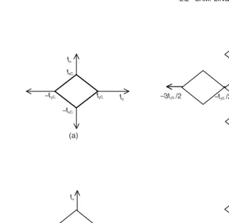
Figure 2.3 Fourier domain illustration of aliasing distortion due to sampling a continuous image: (a) Fourier transform of a continuous lowpass image, (b) Fourier transform of the sampled image with sampling frequencies exactly equal to the respective Nyquist frequencies, (c) Fourier transform of the sampled image with undersampling, and (d) Fourier transform of the sampled image for oversampling.

(42)

frequencies equal to half the sampling frequencies. When the sampling rates are less than the Nyquist rates, the replicas overlap and the portion of the Fourier transform in the region specified by

(−fxC, fxC)×−fyC, fyC

no longer corresponds to that of the continuous image, and therefore, exact recovery is not possible, see Fig-ure 2.3c. In this case, the frequencies above fx S/2 and fy S/2aliasthemselves as low frequencies by folding over and hence the name aliasing distortion. The frequencies fx S/2 and fy S/2 are called thefold overfrequencies. When the sampling rates are greater than the corresponding Nyquist rates, the replicas do not overlap and there is no aliasing distortion as shown in Figure 2.3d.

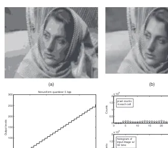
Example 2.1 Read a grayscale image, downsample it by a factor ofM, and

recon-struct the full size image from the downsampled image. Now, prefilter the original image with a lowpass filter and repeat downsampling and reconstruction as before. Discuss the effects. Choose a value of 4 forM.

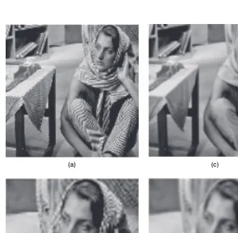
Solution Let us read Barbara image, which is of size 661×628 pixels. Figure 2.4a is the original image downsampled by 4 without any prefiltering. The reconstructed image is shown in Figure 2.4b. The image has been cropped so as to have a man-ageable size. We can clearly see the aliasing distortions in both figures—the patterns in the cloth. Now, we filter the original image with a Gaussian lowpass filter of size 7 ×7 and then downsample it as before. Figures 2.4c,d correspond to the down-sampled and reconstructed images with prefiltering. We see no aliasing distortions in the downsampled and reconstructed images when a lowpass prefiltering is applied before downsampling. However, the reconstructed image is blurry, which is due to lowpass filtering.

% Example2 1.m

% Resamples an original image to study the % effects of undersampling

%

A = imread(’barbara.tif’); [Height,Width,Depth] = size(A); if Depth == 1

f = A; else

f = A(:,:,1); end

% downsample by a factor of M, no prefiltering M = 4;

f1 = f(1:M:Height,1:M:Width);

figure,imshow(f1), title([’Downsampled by ’ num2str(M) ’:No prefiltering’])

f1 = imresize(f1,[Height,Width],’bicubic’);%reconstruct to full size figure,imshow(f1(60:275,302:585))

(43)

% downsample by a factor of M, after prefiltering % use a gaussian lowpass filter

f = imfilter(f,fspecial(’gaussian’,7,2.5),’symmetric’,’same’); f1 = f(1:M:Height,1:M:Width);

figure,imshow(f1), title([’Downsampled by ’ num2str(M) ’ after prefiltering’])

f1 = imresize(f1,[Height,Width],’bicubic’); figure,imshow(f1(60:275,302:585))

title(’Reconstructed from downsampled image: with prefiltering’)

(a) (c)

(d) (b)

(44)

2.2.2 Nonideal Sampling

Practical sampling devices use rectangular pulses of finite width. That is, the sam-pling function is an array of rectangular pulses rather than impulses. Therefore, the sampling function can be written as

s(x,y)=

∞

m=−∞ ∞

n=−∞

p(x₋mx,y₋ny) (2.21)

where p(x,y) is a rectangular pulse of finite extent and of unit area. Then the sam-pling process is equivalent to convolving the continuous image with the pulsep(x,y) and then sampling with a Dirac delta function [1]. The net effect of sampling with a finite-width pulse array is equivalent to prefiltering the image with a lowpass filter corresponding to the pulse p(x,y) followed by ideal sampling. The lowpass filter will blur the image. This is the additional distortion to the aliasing distortion that we discussed above. To illustrate the effect the nonideal sampling has on the sampled image, let us look at the following example.

Example 2.2 Consider an image shown in Figure 2.5a, where the image is a

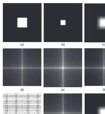
rect-angular array of size 64 ×64 pixels. It is sampled by a rectangular pulse of size 32×32 pixels as shown in Figure 2.5b. The sampled image is shown in Figure 2.5c. We can clearly see the smearing effect of sampling with a rectangular pulse of fi-nite width. The 2D Fourier transforms of the input image, sampling pulse, and the sampled image are shown in Figures 2.5d–f, respectively. Since the smearing effect is equivalent to lowpass filtering, the Fourier transform of the sampled image is a bit narrower than that of the input image. The Fourier transform of an ideal impulse and the Fourier transform of the corresponding sampled image are shown in Figures 2.5g,h, respectively. In contrast to the sampling with a pulse of finite width, we see that the Fourier transform of the ideally sampled image is the same as that of the input image. Finally, the reconstructed image using an ideal lowpass filter is shown in Figure 2.5i. It is identical to the sampled image because we employed sampling with a pulse of finite width.

% Example2 2.m

% Example showing the effect of image sampling with a % finite width pulse

% Two cases are possible: ’delta’ and ’pulse’ % delta corresponds to impulse sampling and pulse % to sampling with finite width pulse.

% image array size is NxN pixels

% actual image area to be sampled is MxM % TxT is the sampling pulse area

samplingType = ’pulse’; % ’delta’ or ’pulse’ N = 256; % array size is NxN

(45)

2.2 SAMPLING A CONTINUOUS IMAGE 31 M = 32; % image pulse width

M1 = N/2 - M + 1; % image beginning point M2 = N/2+M; % image end point

f(M1:M2,M1:M2) = 1; % test image has a value 1 %

p = zeros(N,N); % sampling rectangular pulse if strcmpi(samplingType,’delta’)

p(128,128) = 1; end

if strcmpi(samplingType,’pulse’) T = M/2; % sampling pulse width

T1 = N/2 - T + 1; % sampling pulse beginning point T2 = N/2+T; % sampling pulse end point

p(T1:T2,T1:T2) = 1; % sampling pulse; width = 1/2 of image end

fs = conv2(f,p,’same’); % convolution of image & pulse figure,imshow(f,[]),title(’Input Image’)

figure,imshow(p,[]), title(’Sampling Pulse’) figure,imshow(fs,[]),title(’Sampled Image’) %

figure,imshow(log10(1+5.5*abs(fftshift(fft2(f)))),[]) title(’Fourier Transform of input image’)

if strcmpi(samplingType,’delta’)

figure,imshow(log10(1+1.05*abs(fftshift(fft2(p)))),[]) title(’Fourier Transform of Delta Function’)

end

if strcmpi(samplingType,’pulse’)

figure,imshow(log10(1+5.5*abs(fftshift(fft2(p)))),[]) title(’Fourier Transform of rectangular pulse’) end

%

Fs = fftshift(fft2(fs));

figure,imshow(log10(1+5.5*abs(Fs)),[]) title(’Fourier Transform of sampled image’) % h is the 2D reconstruction filter

%h = (sinc(0.1*pi*(-128:127)))’ * sinc(0.1*pi*(-128:127)); h = (sinc(0.2*pi*(-128:127)))’ * sinc(0.2*pi*(-128:127)); H = fft2(h);

figure,imshow(ifftshift(ifft2(fft2(fs).*H,’symmetric’)),[]) title(’Reconstructed image’)

2.2.3 Nonrectangular Sampling Grids

(46)

(a) (b) (c)

(d) (e) (f)

(g) (h) (i)

Figure 2.5 Effect of nonideal sampling: (a) a 64_× 64 BW image, (b) rectangular sampling image of size 32_×32 pixels, (c) sampled image, (d) 2D Fourier transform of (a), (e) 2D Fourier transform of (b), (f) 2D Fourier transform of the sampled image in (b), (g) 2D Fourier transform of an ideal impulse, (h) 2D Fourier transform of (a) sampled by impulse, and (i) image in (c) obtained by filtering by an ideal lowpass filter.

(47)

2.2 SAMPLING A CONTINUOUS IMAGE 33 especially for motion estimation and compensation, it may be more efficient to em-ploy hexagonal grids for such purposes for better accuracy in motion estimation and higher compression ratio.

Let us briefly describe here the process of converting pixels from rectangular to hexagonal sampling grids and vice versa and illustrate the processes by a couple of examples. The set of points in the (n1, n2)-plane are transformed linearly into the set of points (t1, t2) using the transformation

pendent. For the set of points (t1,t2) to be on a hexagonal sampling grid, the trans-formation takes the form

v₌

Example 2.3 Convert a 256×256 array of pixels of alternating black and white

(BW) dots to a hexagonal sampling grid and display both arrays as images. Assume the sample spacing to be equal to unity.

Solution We will use the linear transformation

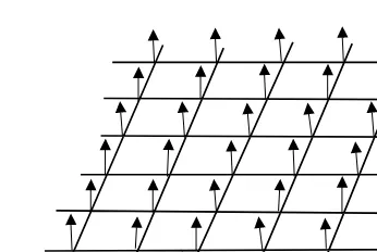
to transform pixels in the rectangular array into the hexagonal array. Note that the range for the hexagonal grid is [(2,512)×(−255,255)]. Figures 2.6a,b show the rectangular and hexagonal sampling grids, respectively, while Figures 2.6c,d cor-respond to the zoomed versions with a zoom factor of 4. The MATLAB code for Example 2.3 is listed below.

Example 2.4 In this example, we will convert the Barbara image from the original

(48)

(d)

(a) (b)

(c)

Figure 2.6 Converting from rectangular to hexagonal sampling grids: (a) pixels on a rectangular grid with unit spacing in both horizontal and vertical directions, (b) pixels on hexagonal grids after applying the transformation in equation (2.22), (c) zoomed version of (a), and (d) zoomed version of (b). In both (c) and (d), the zoom factor is 4.

(a) (b)

(49)

% Example2 3.m

% convert rectangular to hexagonal grid

clear close all

M = 256; N = 256; f = uint8(zeros(N,N)); g = uint8(zeros(M+N,M+N));

% create an image with alternating black & white dots

% for visibility sake, these are R/2xR/2 squares %

R = 2; % pixel replication factor for k = 1:R:M

for l = 1:R:N for k1 = 1:R/2

for l1 = 1:R/2

f(k+k1-1,l+l1-1) = 255; end

end end end

figure,imshow(f), title(’Rectangular grid’) Fig1 = figure;

imshow(f), title(’Rectangular grid’) zoom(Fig1,4)

%

% rectangular to hexagonal transformation V = [1 1; 1 -1];

for n1 = 1:M for n2 = 1:N

t1 = V(1,1)*n1 + V(1,2)*n2; t2 = V(2,1)*n1 + V(2,2)*n2; g(513-t1,256+t2) = f(n1,n2); end

end

figure,imshow(g), title(’Hexagonal grid’) g1 = imcrop(g,[130 130 230 230]);

Fig2 = figure;

imshow(g1), title(’Hexagonal grid’) zoom(Fig2,4)

% Example2 4.m

% convert rectangular to hexagonal grid % using linear transformation

% Sample spacing is DX in the row dimension % and DY in the column dimension

% transformation is [t1 t2]’ = V*[n1 n2]’; % where V = [DX DY; DX -DY];

% In our example we assume DX = DY = 1; clear

(50)

g = uint8(zeros(M+N,M+N));% transformed image twice as big as the input

%

% Convert rectangular to hexagonal sampling

V = [1 1; 1 -1]; % rectangular to hexagonal transformation for n1 = 1:M % Now revert to rectangular grid

VI = inv(V);

f1 = uint8(zeros(M+N,M+N)); for t1 = 2:M+N

%for t2 = -N+1:N-1 for t2 = -N+1:M-1

n1 = floor(VI(1,1)*t1 + VI(1,2)*t2); n2 = floor(VI(2,1)*t1 + VI(2,2)*t2); %f1(n1+M/2,n2+N/2) = g(N2+1-t1,M+t2);

%f1(n1+round((N-1)/2),n2+round((M-1)/2)) = g(N2+1- t1,M+t2); f1(n1+round((N-1)/2),n2+round((M-1)/2)) = g(M+N+1- t1,N+t2); end

end

(51)

2.3 IMAGE QUANTIZATION 37

2.3 IMAGE QUANTIZATION

As indicated in Figure 2.1, the image samples have a continuum of values. That is, the samples are analog and must be represented in digital format for storage or transmis-sion. Because the number of bits (binary digits) for representing each image sample is limited—typically 8 or 10 bits, the analog samples must first bequantized to a finite number of levels and then the particular level must be coded in binary number. Because the quantization process compresses the continuum of analog values to a fi-nite number of discrete values, some distortion is introduced in the displayed analog image. This distortion is known asquantization noiseand might manifest as patches, especially in flat areas. This is also known ascontouring.

In simple terms, a scalar quantizer observes an input analog sample and outputs a numerical value. The output numerical value is a close approximation to the input value. The output values are predetermined corresponding to the range of the input and the number of bits allowed in the quantizer. Formally, we define a scalar quan-tizerQ(·) to be a mapping of inputdecision intervals_{dk,k=1,2, . . . , L+1}to output orreconstruction levels_{rk,k₌1, . . . , L_}. Thus,

Q(x)₌xˆ ₌rk (2.24)

We assume that the quantizer output levels are chosen such that

r1≺r2≺ · · · ≺rL (2.25)

The number of bits required to address any one of the output levels is

B₌log2L

(bits) (2.26)

where⌈x_⌉is the nearest integer equal to or larger thanx.

A design of a quantizer amounts to specifying the decision intervals and corre-sponding output levels and a mapping rule. Since there are many possibilities to partition the input range, we are interested in the optimal quantizer that minimizes a certain criterion or cost function. In the following section, we will develop the algorithm for such an optimal quantizer.

2.3.1 Lloyd–Max Quantizer

(52)

such that the MSE is minimized:

MSE₌E

In equation (2.27),Edenotes the expectation operator. Note that the output value is constant and equal torj over the input range

dj,dj+1

. Therefore, equation (2.27) can be written as

MSE=

Minimization of equation (2.28) is obtained by differentiating the MSE with re-spect todjandrjand setting the partial derivatives to zero. Thus,

∂MSE

From equation (2.29a), we obtain

Becauserj ≻rj−1, equation (2.30) after simplification yields

dj =

rj+rj−1

2 (2.31a)

From equation (2.29b), we get

rj =

(53)

2.3 IMAGE QUANTIZATION 39 output levels for given input pdf andL. These tables assume that the input analog signal to have unit variance. To obtain the optimal quantizer decision intervals and output levels for an analog signal having a specific variance, one must multiply the tabulated values by the standard deviation of the actual signal.

2.3.2 Uniform Quantizer

When the pdf of the analog sample is uniform, the decision intervals and output levels of the Lloyd–Max quantizer can be computed analytically as shown below. In this case, the decision intervals are all equal as well as the intervals between the output levels and the quantizer is called auniformquantizer. The uniform pdf of the input image is given by

px(x)= 1 xmax−xmin =

1 dL₊1−d1

(2.32)

Using equation (2.32) in (2.31b), we get

rj ₌

dj+1−dj 2

2 (xmax−xmin)

dj+1−dj (xmax−xmin)

=

dj+1+dj

2 (2.33)

From equations (2.33) and (2.31a), we can write

dj+1−dj =dj−dj−1=,2≤ j ≤L (2.34)

From the above equation, we see that the interval between any two consecutive deci-sion boundaries is the same and equal to the quantization step size. Using equation (2.34), we can also expressdjin terms ofdj+1anddj−1as

dj=

dj+1+dj−1

2 (2.35)

The quantization step size of the uniform quantizer is related to the number of levels Lor the number of bitsB, as given in equation (2.36).

₌ xmax−xmin

L =

dL+1−d1

(54)

Finally, combining equations (2.33) and (2.34) we can express the reconstruction levels by

rj ₌ dj++dj

2 =dj+

2 (2.37)

From equation (2.37), we find that the intervals between the output levels are also equal to. Thus, the design of the optimal or Lloyd–Max quantizer for a signal with uniform distribution is carried out as follows:

1. Divide the input range (xmin,xmax) intoLequal stepsas given in equation (2.36) withd1 =xminanddL+1=xmax.

2. Determine theLoutput levels from equation (2.37).

3. Quantize a samplexaccording toQ(x)=rj,ifdj≤x≺dj+1.

2.3.3 Quantizer Performance

For the uniform quantizer, the quantization errore₌x₋xˆhas the range (−2,

2), and it is uniformly distributed as well. Therefore, the MSEσ_q2for the uniform quan-tizer can be found from

σ_q2₌ 1

/2

−/2

e2de₌ 2

12 (2.38)

We can express the performance of a uniform quantizer in terms of the achievable signal-to-noise ratio (SNR). The noise power due to quantization is given by equa-tion (2.38). The variance of a uniformly distributed random variable in the range

(xmin,xmax) is evaluated from

σ_x2₌

xmax

xmin

(x₋µ)2px(x)d x= 1 (xmax−xmin)

xmax

xmin

(x₋µ)2d x (2.39)

Whereµis the average value of the input signal, as given by

µ₌ 1

(xmax−xmin) xmax

xmin

xd x₌ xmax+xmin

(55)

2.3 IMAGE QUANTIZATION 41 Using equation (2.40) in (2.39) and with some algebraic manipulation, we find that the signal variance equals

σ_x2₌ (xmax−xmin) 2

12 (2.41)

Therefore, the SNR of a uniform quantizer is found to be

SNR= σ 2 x

σ2 q

= (xmax−xmin) 2

2 =

(xmax−xmin)2 (xmax−xmin)2

22B

=22B (2.42)

In dB, aB-bit uniform quantizer yields an SNR of

SNR=10 log 22B ∼₌6B (dB) (2.43) From equation (2.43), we find that each additional bit in the quantizer improves its SNR by 6 dB. Stated in another way, the Lloyd–Max quantizer for signals with uniform pdf gives an SNR of 6 dB/bit of quantization.

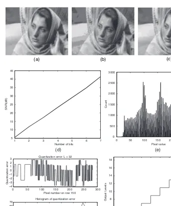
Example 2.5 Read a BW image with 8 bits/pixel and requantize it toBbits/pixel

using a uniform quantizer. Display both the original and requantized images and observe the differences, if any. Plot the SNR in dB due to quantization noise. For display purpose, assumeBto be 3 and 5 bits. For plotting, varyBfrom 1 to 7 bits.

Solution For the uniform quantizer withB bits of quantization, the quantization step size is found to be

₌255 2B

Then, the decision boundaries and output levels can be calculated from

dk=dk−1+,2≤k≤ L+1; d1=0,dL+1=255 rk₌dk₊

2,1≤k≤L

After calculating the decision boundaries and reconstruction levels, the B-bit quantizer assigns to each input pixel an out value using the rule:

outputrkifdk_≤input≺dk₊1,1≤k≤L

(56)

3 Quantization error: L = 32

Pixel number on row 150

Quantization error

Histogram of quantization error