Signals and Systems with MATLAB

(1)

(2)

(3)

(4)

Won Y. Yang

·

Tae G. Chang

·

Ik H. Song

·

Yong S. Cho

·

Jun Heo

·

Won G. Jeon

·

Jeong W. Lee

·

Jae K. Kim

Signals and Systems

with MATLAB

R

(5)

Limits of Liability and Disclaimer of Warranty of Software

The reader is expressly warned to consider and adopt all safety precautions that might be indicated by the activities herein and to avoid all potential hazards. By following the instructions contained herein, the reader willingly assumes all risks in connection with such instructions.

The authors and publisher of this book have used their best efforts and knowledge in preparing this book as well as developing the computer programs in it. However, they make no warranty of any kind, expressed or implied, with regard to the programs or the documentation contained in this book. Accordingly, they shall not be liable for any incidental or consequential damages in connection with, or arising out of, the readers’ use of, or reliance upon, the material in this book.

Questions about the contents of this book can be mailed to wyyang.53@hanmail.net. Program files in this book can be downloaded from the following website:

<http://wyyang53.com.ne.kr/>

MATLABR _{and Simulink}R _{are registered trademarks of The MathWorks, Inc. For} MATLAB and Simulink product information, please contact:

The MathWorks, Inc. 3 Apple Hill Drive

Natick, MA 01760-2098 USA

: 508-647-7000, Fax: 508-647-7001 E-mail: info@mathworks.com Web: www.mathworks.com

ISBN 978-3-540-92953-6 e-ISBN 978-3-540-92954-3 DOI 10.1007/978-3-540-92954-3

Springer Dordrecht Heidelberg London New York

Library of Congress Control Number: 2009920196 c

Springer-Verlag Berlin Heidelberg 2009

This work is subject to copyright. All rights are reserved, whether the whole or part of the material is concerned, specifically the rights of translation, reprinting, reuse of illustrations, recitation, broadcasting, reproduction on microfilm or in any other way, and storage in data banks. Duplication of this publication or parts thereof is permitted only under the provisions of the German Copyright Law of September 9, 1965, in its current version, and permission for use must always be obtained from Springer. Violations are liable to prosecution under the German Copyright Law.

The use of general descriptive names, registered names, trademarks, etc. in this publication does not imply, even in the absence of a specific statement, that such names are exempt from the relevant protective laws and regulations and therefore free for general use.

Cover design:WMXDesign GmbH, Heidelberg Printed on acid-free paper

(6)

To our parents and families

who love and support us

and

(7)

(8)

Preface

This book is primarily intended for junior-level students who take the courses on ‘signals and systems’. It may be useful as a reference text for practicing engineers and scientists who want to acquire some of the concepts required for signal process-ing. The readers are assumed to know the basics about linear algebra, calculus (on complex numbers, differentiation, and integration), differential equations, Laplace transform, and MATLABR_{. Some knowledge about circuit systems will be helpful.} Knowledge in signals and systems is crucial to students majoring in Electrical Engineering. The main objective of this book is to make the readers prepared for studying advanced subjects on signal processing, communication, and control by covering from the basic concepts of signals and systems to manual-like introduc-tions of how to use the MATLABR _{and Simulink}R _{tools for signal analysis and} filter design. The features of this book can be summarized as follows:

1. It not only introduces the four Fourier analysis tools, CTFS (continuous-time Fourier series), CTFT (continuous-time Fourier transform), DFT (discrete-time Fourier transform), and DTFS (discrete-time Fourier series), but also illuminates the relationship among them so that the readers can realize why only the DFT of the four tools is used for practical spectral analysis and why/how it differs from the other ones, and further, think about how to reduce the difference to get better information about the spectral characteristics of signals from the DFT analysis. 2. Continuous-time and discrete-time signals/systems are presented in parallel to

save the time/space for explaining the two similar ones and increase the under-standing as far as there is no concern over causing confusion.

3. It covers most of the theoretical foundations and mathematical derivations that will be used in higher-level related subjects such as signal processing, commu-nication, and control, minimizing the mathematical difficulty and computational burden.

4. Most examples/problems are titled to illustrate key concepts, stimulate interest, or bring out connections with any application so that the readers can appreciate what the examples/problems should be studied for.

5. MATLABR _{is integrated extensively into the text with a dual purpose. One} is to let the readers know the existence and feel the power of such software tools as help them in computing and plotting. The other is to help them to

(9)

viii Preface

realize the physical meaning, interpretation, and/or application of such concepts as convolution, correlation, time/frequency response, Fourier analyses, and their results, etc.

6. The MATLABR _{commands and Simulink}R _{blocksets for signal processing} application are summarized in the appendices in the expectation of being used like a manual. The authors made no assumption that the readers are proficient in MATLABR _{. However, they do not hide their expectation that the readers will} get interested in using the MATLABR _{and Simulink}R _{for signal analysis and} filter design by trying to understand the MATLABR _{programs attached to some} conceptually or practically important examples/problems and be able to modify them for solving their own problems.

The contents of this book are derived from the works of many (known or unknown) great scientists, scholars, and researchers, all of whom are deeply appre-ciated. We would like to thank the reviewers for their valuable comments and suggestions, which contribute to enriching this book.

We also thank the people of the School of Electronic & Electrical Engineering, Chung-Ang University for giving us an academic environment. Without affections and supports of our families and friends, this book could not be written. Special thanks should be given to Senior Researcher Yong-Suk Park of KETI (Korea Elec-tronics Technology Institute) for his invaluable help in correction. We gratefully acknowledge the editorial and production staff of Springer-Verlag, Inc. including Dr. Christoph Baumann and Ms. Divya Sreenivasan, Integra.

Any questions, comments, and suggestions regarding this book are welcome. They should be sent to wyyang53@hanmail.net.

Seoul, Korea Won Y. Yang

(10)

E MATLAB. . . 421

E.1 Convolution and Deconvolution . . . 423

E.2 Correlation . . . 424

E.3 CTFS (Continuous-Time Fourier Series) . . . 425

E.4 DTFT (Discrete-Time Fourier Transform) . . . 425

E.5 DFS/DFT (Discrete Fourier Series/Transform) . . . 425

E.6 FFT (Fast Fourier Transform) . . . 426

E.7 Windowing . . . 427

E.8 Spectrogram (FFT with Sliding Window) . . . 427

E.9 Power Spectrum . . . 429

E.10 Impulse and Step Responses . . . 430

E.11 Frequency Response . . . 433

E.12 Filtering . . . 434

(16)

E.13.1 Analog Filter Design . . . 436

E.13.2 Digital Filter Design – IIR (Infinite-duration Impulse Response) Filter . . . 437

E.13.3 Digital Filter Design – FIR (Finite-duration Impulse Response) Filter . . . 438

E.14 Filter Discretization . . . 441

E.15 Construction of Filters in Various Structures Using dfilt() . . . 443

E.16 System Identification from Impulse/Frequency Response . . . 447

E.17 Partial Fraction Expansion and (Inverse) Laplace/z-Transform . . . 449

E.18 Decimation, Interpolation, and Resampling . . . 450

E.19 Waveform Generation . . . 452

E.20 Input/Output through File . . . 452

F SimulinkR . . . 453

Index . . . 461

Index for MATLAB routines. . . 467

Index for Examples. . . 471

(17)

Chapter 1

Signals and Systems

Contents

1.1 Signals . . . 2

1.1.1 Various Types of Signal . . . 2

1.1.2 Continuous/Discrete-Time Signals . . . 2

1.1.3 Analog Frequency and Digital Frequency . . . 6

1.1.4 Properties of the Unit Impulse Function and Unit Sample Sequence . . . 8

1.1.5 Several Models for the Unit Impulse Function . . . 11

1.2 Systems . . . 12

1.2.1 Linear System and Superposition Principle . . . 13

1.2.2 Time/Shift-Invariant System . . . 14

1.2.3 Input-Output Relationship of Linear Time-Invariant (LTI) System . . . 15

1.2.4 Impulse Response and System (Transfer) Function . . . 17

1.2.5 Step Response, Pulse Response, and Impulse Response . . . 18

1.2.6 Sinusoidal Steady-State Response and Frequency Response . . . 19

1.2.7 Continuous/Discrete-Time Convolution . . . 22

1.2.8 Bounded-Input Bounded-Output (BIBO) Stability . . . 29

1.2.9 Causality . . . 30

1.2.10 Invertibility . . . 30

1.3 Systems Described by Differential/Difference Equations . . . 31

1.3.1 Differential/Difference Equation and System Function . . . 31

1.3.2 Block Diagrams and Signal Flow Graphs . . . 32

1.3.3 General Gain Formula – Mason’s Formula . . . 34

1.3.4 State Diagrams . . . 35

1.4 Deconvolution and Correlation . . . 38

1.4.1 Discrete-Time Deconvolution . . . 38

1.4.2 Continuous/Discrete-Time Correlation . . . 39

1.5 Summary . . . 45

Problems . . . 45

In this chapter we introduce the mathematical descriptions of signals and sys-tems. We also discuss the basic concepts on signal and system analysis such as linearity, time-invariance, causality, stability, impulse response, and system function (transfer function).

W.Y. Yang et al.,Signals and Systems with MATLABR_,

DOI 10.1007/978-3-540-92954-3 1,C Springer-Verlag Berlin Heidelberg 2009

(18)

1.1 Signals

1.1.1 Various Types of Signal

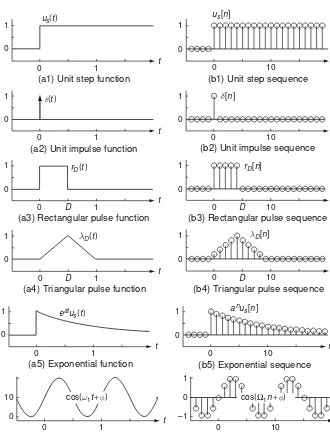
Asignal, conveying information generally about the state or behavior of a physical system, is represented mathematically as a function of one or more independent variables. For example, a speech signal may be represented as an amplitude function of time and a picture as a brightness function of two spatial variables. Depending on whether the independent variables and the values of a signal are continuous or discrete, the signal can be classified as follows (see Fig. 1.1 for examples):

- Continuous-time signal x(t): defined at a continuum of times.

- Discrete-time signal (sequence) x[n]=x(nT): defined at discrete times. - Continuous-amplitude(value) signal xc: continuous in value (amplitude).

- Discrete-amplitude(value) signal xd: discrete in value (amplitude).

Here, the bracket [] indicates that the independent variable n takes only integer values. A continuous-time continuous-amplitude signal is called ananalog signal

while a discrete-time discrete-amplitude signal is called adigital signal. The ADC (analog-to-digital converter) converting an analog signal to a digital one usually performs the operations of sampling-and-hold, quantization, and encoding. How-ever, throughout this book, we ignore the quantization effect and use “discrete-time signal/system” and “digital signal/system” interchangeably.

Continuous-time continuous-amplitude

signal

x(t)

sampling at t=nT T: sample period

T

hold

(a) (b) (c) (d) (e)

A/D conversion D/A conversion Continuous-time

continuous-amplitude sampled signal

x∗(t)

Discrete-time discrete-amplitude

signal

x_d[n]

Continuous-time discrete-amplitude

signal

x_d(t)

Continuous-time continuous-amplitude

signal

x(t)

Fig. 1.1 Various types of signal

1.1.2 Continuous/Discrete-Time Signals

(19)

1.1 Signals 3

0

(a1) Unit step function

u_s(t )

t 1

1

(a2) Unit impulse function

δ(t )

t

0 1

(a3) Rectangular pulse function

r_D(t )

t

0 D 1

0 1

(a4) Triangular pulse function

λ_D(t )

t

0 D 1

0 1

(a5) Exponential function

eat_u

s(t )

t

0 1

(b2) Unit impulse sequence δ[n ]

n

0 10

0 1

(b3) Rectangular pulse sequence

r_D[n]

n

0 D 10

0 1

(b1) Unit step sequence

u_s[n]

n

0 10

0 1

(b4) Triangular pulse sequence λD[n]

n

0 D 10

0 1

(b5) Exponential sequence

anus[n ]

n

0 10

0 1

(a6) Real sinusoidal function

cos(ω₁t+φ)

t

0 1

0 10

(b6) Real sinusoidal sequence

cos(Ω1n+φ)

n

0 10

0

–1 1

Fig. 1.2 Some continuous–time and discrete–time signals

1.1.2.1a Unit step function 1.1.2.1b Unit step sequence

us(t)=

1 fort≥0

0 fort<0 (1.1.1a) us[n]=

1 forn≥0

(20)

Im

Re

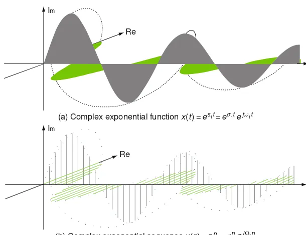
(a) Complex exponential function x(t )=e

s₁t₌_eσ₁t _e

jω₁t

t

n

(b) Complex exponential sequence x(n)=z1n = r1ne

j Ω

1n

Fig. 1.3 Continuous–time/discrete–time complex exponential signals

(cf.) A delayed and scaled step function (cf.) A delayed and scaled step sequence

Aus(t−t0)=

A fort≥t0 0 fort<t0

Aus[n−n0]=

A forn≥n0 0 forn<n0

1.1.2.2a Unit impulse function 1.1.2.2b Unit sample or impulse sequence

δ(t)= d

dtus(t)=

∞ fort =0

0 fort =0

(1.1.2a)

δ[n]=

1 forn =0

0 forn =0 (1.1.2b)

(cf.) A delayed and scaled impulse function

(cf.) A delayed and scaled impulse sequence

Aδ(t−t0)=

A∞ fort =t0

0 fort =t0

Aδ[n−n0]=

A for n = n0

(21)

1.1 Signals 5

(cf.) Relationship betweenδ(t) andus(t)

δ(t)= d

dtus(t) (1.1.3a) us(t)=

t

−∞

δ(τ)dτ (1.1.4a)

1.1.2.3a Rectangular pulse function

rD(t)=us(t)−us(t−D) (1.1.5a)

=

1 for 0≤t<D(D: duration)

0 elsewhere

1.1.2.4a Unit triangular pulse function

λD(t)=

1− |t−D|/D for|t−D| ≤D

0 elsewhere

(1.1.6a) 1.1.2.5a Real exponential function

x(t)=eatus(t)=

eat fort≥0 0 fort<0

(1.1.7a)

1.1.2.6a Real sinusoidal function

x(t)=cos(ω1t+φ)=Re{ej(ω1t+φ)_} = 1

2

ejφejω1t₊_e−jφ_e−jω1t (1.1.8a)

1.1.2.7a Complex exponential function

x(t)=es1t₌_eσ1t_ejω1t_with _s

1=σ1+jω1 (1.1.9a)

Note that σ1 determines the changing rate or the time constant and ω1 the oscillation frequency.

1.1.2.8a Complex sinusoidal function

x(t)=ejω1t₌_cos(_ω1_t₎₊_j_sin(_ω1_t₎ (1.1.10a)

(cf) Relationship betweenδ[n] andus[n]

δ[n]=us[n]−us[n−1] (1.1.3b)

us[n]=

n

m=−∞δ[m] (1.1.4b)

1.1.2.3b Rectangular pulse sequence

rD[n]=us[n]−us[n−D] (1.1.5b)

=

1 for 0≤n <D(D: duration)

0 elsewhere

1.1.2.4b Unit triangular pulse sequence

λD[n]=

1− |n+1−D|/Dfor|n+1−D| ≤D−1 0 elsewhere

(1.1.6b) 1.1.2.5b Real exponential sequence

x[n]=anus[n]=

an _for_n_≥₀

0 forn<0 (1.1.7b) 1.1.2.6b Real sinusoidal sequence

x[n]=cos(Ω1n+φ)=Reej(Ω1n+φ) = 1

2

ejφejΩ1n₊_e−jφ_e−jΩ1n

(1.1.8b)

1.1.2.7b Complex exponential function

x[n]=zn₁ =r₁nejΩ1n _with _z

1=r1ejΩ1 (1.1.9b)

Note that r1 determines the changing rate andΩ1the oscillation frequency.

1.1.2.8b Complex sinusoidal sequence

x[n]=ejΩ1n ₌_cos(_Ω

(22)

1.1.3 Analog Frequency and Digital Frequency

A continuous-time signalx(t) isperiodicwithperiod PifPis generally the smallest positive value such thatx(t+P)=x(t). Let us consider a continuous-time periodic signal described by

x(t)=ejω1t _(1.1.11)

Theanalogorcontinuous-time(angular)frequency1_{of this signal is}_ω1_{[rad/s] and} its period is

P =2π

ω1[s] (1.1.12)

where

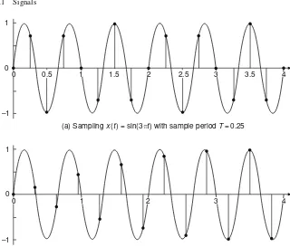
ejω1(t+P)₌_ejω1t_∀_t ₍_∵ _ω1_P ₌₂_π _⇒_ejω1P ₌₁₎ _(1.1.13) If we sample the signalx(t)=ejω1t _{periodically at}_t ₌_nT_{, we get a} discrete-time signal

x[n]=ejω1nT ₌_ejΩ1n_with_Ω

1=ω1T (1.1.14)

Will this signal be periodic inn? You may well think that x[n] is also periodic for any sampling intervalT since it is obtained from the samples of a continuous-time periodic signal. However, the discrete-continuous-time signalx[n] is periodic only when the sampling interval T is the continuous-time period P multiplied by a rational number, as can be seen from comparing Fig. 1.4(a) and (b). If we samplex(t) = ejω1t_{to get}_x_[_n_]₌_ejω1nT ₌_ejΩ1n_{with a sampling interval}_T ₌_{m P}_/_N_[s/sample] where the two integersmandN are relatively prime (coprime), i.e., they have no common divisor except 1, the discrete-time signal x[n] is also periodic with the

digitalordiscrete-time frequency Ω1=ω1T =ω1

m P N =

m

N2π[rad/sample] (1.1.15)

The period of the discrete-time periodic signalx[n] is

N = 2mπ Ω1

[sample], (1.1.16)

where

ejΩ1(n+N) =ejΩ1n_ej2mπ ₌_ejΩ1n_∀_n _(1.1.17)

1_{Note that we call the angular or radian frequency measured in [rad/s] just the frequency}

(23)

1.1 Signals 7

1 2 3

1

0 0

0 1 2 3 4

0.5 1.5 2.5

(a) Sampling x(t) = sin(3πt) with sample period T=0.25

(b) Sampling x(t) = sin(3πt) with sample period T = 1/π

3.5 4 t

t –1

1

0

–1

Fig. 1.4 Sampling a continuous–time periodic signal

This is the counterpart of Eq. (1.1.12) in the discrete-time case. There are several observations as summarized in the following remark:

Remark 1.1Analog (Continuous-Time) Frequency and Digital (Discrete-Time) Frequency

(1) In order for a discrete-time signal to be periodic with period N (being an integer), the digital frequencyΩ1must beπ times a rational number.

(2) The periodN of a discrete-time signal with digital frequencyΩ1 is the mini-mum positive integer to be multiplied byΩ1to make an integer times 2π like 2mπ (m: an integer).

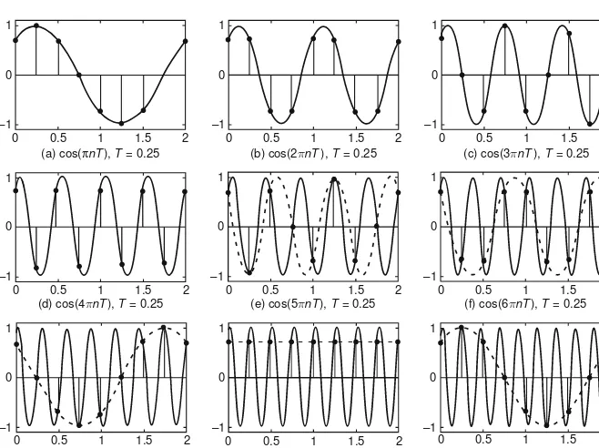
(3) In the case of a continuous-time periodic signal with analog frequencyω1, it can be seen to oscillate with higher frequency asω1 increases. In the case of a discrete-time periodic signal with digital frequencyΩ1, it is seen to oscillate faster as Ω1 increases from 0 to π (see Fig. 1.5(a)–(d)). However, it is seen to oscillate rather slower asΩ1 increases fromπ to 2π (see Fig. 1.5(d)–(h)). Particularly withΩ1 =2π(Fig. 1.5(h)) or 2mπ, it is not distinguishable from a DC signal withΩ1 =0. The discrete-time periodic signal is seen to oscillate faster asΩ1 increases from 2π to 3π (Fig. 1.5(h) and (i)) and slower again as

(24)

1

0

–1

1

0

–1

1

0

–1

1

0

–1

1

0

–1 1

0

–1

1

0

–1 1

0

–1

1

0

–1

0 0.5

(a) cos(πnT), T = 0.25 (b) cos(2πnT), T = 0.25 (c) cos(3πnT), T = 0.25

(d) cos(4πnT), T = 0.25 (e) cos(5πnT), T = 0.25 (f) cos(6πnT), T = 0.25

(g) cos(7πnT), T = 0.25 (h) cos(8πnT), T = 0.25 (i) cos(9πnT), T = 0.25

1 1.5 2

0 0.5 1 1.5 2

0 0.5 1 1.5 2 0 0.5 1 1.5 2 0 0.5 1 1.5 2

0 0.5 1 1.5 2 0 0.5 1 1.5 2

Fig. 1.5 Continuous–time/discrete–time periodic signals with increasing analog/digital frequency

This implies that the frequency characteristic of a discrete-time signal is peri-odic with period 2π in the digital frequencyΩ. This is becauseejΩ1n _{is also} periodic with period 2πinΩ1, i.e.,ej(Ω1+2mπ)n =ejΩ1nej2mnπ =ejΩ1n for any integerm.

(4) Note that if a discrete-time signal obtained from sampling a continuous-time periodic signal has the digital frequency higher than π [rad] (in its absolute value), it can be identical to a lower-frequency signal in discrete time. Such a phenomenon is calledaliasing, which appears as the stroboscopic effect or the wagon-wheel effect that wagon wheels, helicopter rotors, or aircraft propellers in film seem to rotate more slowly than the true rotation, stand stationary, or even rotate in the opposite direction from the true rotation (the reverse rotation effect).[W-1]

1.1.4 Properties of the Unit Impulse Function

and Unit Sample Sequence

In Sect. 1.1.2, theunit impulse, also called theDirac delta, function is defined by Eq. (1.1.2a) as

δ(t)= d

dtus(t)=

∞ fort=0

(25)

1.1 Signals 9

Several useful properties of the unit impulse function are summarized in the follow-ing remark:

Remark 1.2aProperties of the Unit Impulse Functionδ(t)

(1) The unit impulse functionδ(t) has unity area aroundt =0, which means

+∞

−∞

δ(τ)dτ =

0+

0−

δ(τ)dτ =1 (1.1.19)

∵ 0+

−∞

δ(τ)dτ −

0−

−∞

δ(τ)dτ(1.=1.4a)us(0+)−us(0−)=1−0=1

(2) The unit impulse functionδ(t) is symmetric aboutt =0, which is described by

δ(t)=δ(−t) (1.1.20)

(3) The convolution of a time functionx(t) and the unit impulse functionδ(t) makes the function itself:

x(t)∗δ(t) (A=.17)

definition of convolution integral

+∞

−∞

x(τ)δ(t−τ)dτ =x(t) (1.1.21) ⎛

⎝

∵+∞

−∞x(τ)δ(t−τ)dτ

δ(t−τ)=0 for onlyτ=t

= +∞

−∞x(t)δ(t−τ)dτ

x(t) independent ofτ

= x(t)+∞

−∞δ(t−τ)dτ

t−τ→t′

= x(t)t−∞

t+∞δ(t

′₎₍₋_dt′₎₌_x₍_t₎t+∞

t−∞δ(t

′₎_dt′₌_x₍_t₎+∞

−∞δ(τ)dτ

(1.1.19)

= x(t)

⎞

⎠

What about the convolution of a time functionx(t) and a delayed unit impulse functionδ(t−t1)? It becomes the delayed time functionx(t−t1), that is,

x(t)∗δ(t−t1)=

+∞

−∞

x(τ)δ(t−τ−t1)dτ =x(t−t1) (1.1.22)

What about the convolution of a delayed time functionx(t−t2) and a delayed unit impulse functionδ(t−t1)? It becomes another delayed time functionx(t−

t1−t2), that is,

x(t−t2)∗δ(t−t1)=

+∞

−∞

x(τ −t2)δ(t−τ−t1)dτ =x(t−t1−t2) (1.1.23)

Ifx(t)∗y(t)=z(t), we have

x(t−t1)∗y(t−t2)=z(t−t1−t2) (1.1.24) However, withtreplaced witht−t1on both sides, it does not hold, i.e.,

(26)

(4) The unit impulse functionδ(t) has thesamplingorsifting propertythat

+∞

−∞

x(t)δ(t−t1)dt

δ(t−t1)=0 for onlyt=t1 = x(t1)

+∞

−∞

δ(t−t1)dt (1.1.19)

= x(t1)

(1.1.25)

This property enables us to sample or sift the sample value of a continuous-time signalx(t) att =t1. It can also be used to model a discrete-time signal obtained from sampling a continuous-time signal.

In Sect. 1.1.2, the unit-sample, also called the Kronecker delta, sequence is defined by Eq. (1.1.2b) as

δ[n]=

1 forn =0

0 forn =0 (1.1.26)

This is the discrete-time counterpart of the unit impulse functionδ(t) and thus is also called the discrete-time impulse. Several useful properties of the unit-sample sequence are summarized in the following remark:

Remark 1.2bProperties of the Unit-Sample Sequenceδ[n]

(1) Like Eq. (1.1.20) for the unit impulseδ(t), the unit-sample sequenceδ[n] is also symmetric aboutn=0, which is described by

δ[n]=δ[−n] (1.1.27)

(2) Like Eq. (1.1.21) for the unit impulseδ(t), the convolution of a time sequence

x[n] and the unit-sample sequenceδ[n] makes the sequence itself:

x[n]∗δ[n]definition of convolution sum= ∞

m=−∞x[m]δ[n−m]=x[n] (1.1.28)

⎛

⎜ ⎜ ⎜ ⎜ ⎜ ⎜ ⎝

∵∞

m=−∞x[m]δ[n−m]

δ[n−m]=0 for onlym=n

= ∞

m=−∞x[n]δ[n−m]

x[n] independent ofm

= x[n]∞

m=−∞δ[n−m]

δ[n−m]=0 for onlym=n

= x[n]δ[n−n](1.1=.26)x[n]

⎞

(27)

1.1 Signals 11

(3) Like Eqs. (1.1.22) and (1.1.23) for the unit impulseδ(t), the convolution of a time sequence x[n] and a delayed unit-sample sequenceδ[n−n1] makes the delayed sequencex[n−n1]:

x[n]∗δ[n−n1]=

∞

m=−∞x[m]δ[n−m−n1]=x[n−n1] (1.1.29)

x[n−n2]∗δ[n−n1]=

∞

m=−∞x[m−n2]δ[n−m−n1]=x[n−n1−n2]

(1.1.30)

Also like Eq. (1.1.24), we have

x[n]∗y[n]=z[n]⇒x[n−n1]∗y[n−n2]=z[n−n1−n2] (1.1.31) (4) Like (1.1.25), the unit-sample sequenceδ[n] has thesamplingorsifting

prop-ertythat

∞

n=−∞x[n]δ[n−n1]=

∞

n=−∞x[n1]δ[n−n1]=x[n1] (1.1.32)

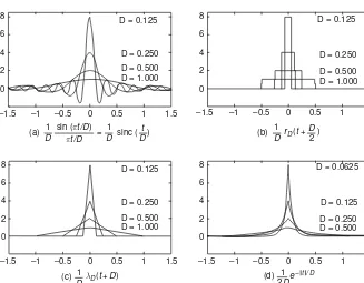
1.1.5 Several Models for the Unit Impulse Function

As depicted in Fig. 1.6(a)–(d), the unit impulse function can be modeled by the limit of various functions as follows:

−δ(t)= lim

D→0+

1

D

sin(πt/D)

πt/D =Dlim→0+

1

Dsinc(t/D)

π/D→w

= lim

w→∞

w π

sin(wt) wt

(1.1.33a)

−δ(t)= lim

D→0+

1

DrD

t+D

2

(1.1.33b)

−δ(t)= lim

D→0+

1

DλD(t+D) (1.1.33c)

−δ(t)= lim

D→0+

1 2De

−|t|/D

(1.1.33d)

Note that scaling up/down the impulse function horizontally is equivalent to scaling it up/down vertically, that is,

δ(at)= 1

|a|δ(t) (1.1.34)

(28)

8 _{D = 0.125} D = 0.250 D = 0.500 D = 1.000

D = 0.125 D = 0.250 D = 0.500 D = 1.000

D = 0.0625 D = 0.125 D = 0.250 D = 0.500 6

4 2 0

8 6 4 2 0 –1.5 –1 –0.5 0 0.5 1 1.5

8 6 4 2 0

–1.5 –1 –0.5 0 0.5 1 1.5 8 6 4 2 0

–1.5 –1 –0.5 0 0.5 1 1.5 –1.5 –1 –0.5 0 0.5 1 1.5

D 2

(b) rD(t + )

1 D

D

(c) 1 λD (t+D)

(a) 1 sin (πt/D)

πt/D D

1

sinc ( ) =

D t D

e– t/D

2D

(d) 1

Fig. 1.6 Various models of the unit impulse functionδ(t)

δ(at)(1.1=.33a) lim

D→0+

1

D

sin(πat/D)

πat/D =D/|lima|→0+

1

|a|(D/|a|)

sin(πt/(D/a)) πt/(D/a)

D/|a|→D′

= 1

|a|Dlim′_→₀+

1

D′

sin(πt/D′₎

πt/D′

(1.1.33a)

= 1

|a|δ(t)

On the other hand, the unit-sample or impulse sequenceδ[n] can be written as

δ[n]= sin(πn)

πn =sinc(n) (1.1.35)

where thesincfunction is defined as

sinc(x)= sin(πx)

πx (1.1.36)

1.2 Systems

(29)

1.2 Systems 13

the input the output

(a) A continuous−time system (b) A discrete−time system

G y(t) = G{x(t)} G

x(t)

the input the output

y[n] = G{x[n]}

x[n]

Fig. 1.7 A description of continuous–time and discrete–time systems

multiple-output(MIMO) system. Asingle-input multiple-output(SIMO) system and amultiple-input single-output(MISO) system can also be defined in a similar way. For example, a spring-damper-mass system is a mechanical system whose output to an input force is the displacement and velocity of the mass. Another example is an electric circuit whose inputs are voltage/current sources and whose outputs are voltages/currents/charges in the circuit. A mathematical operation or a com-puter program transforming input argument(s) (together with the initial conditions) into output argument(s) as a model of a plant or a process may also be called a system.

A system is called a continuous-time/discrete-time system if its input and output are both continuous-time/discrete-time signals. Continuous-time/discrete-time sys-tems with the input and output are often described by the following equations and the block diagrams depicted in Fig. 1.7(a)/(b).

Continuous-time system

x(t)G→{}y(t); y(t)=G{x(t)}

Discrete-time system

x[n]→G{}y[n]; y[n]=G{x[n]}

1.2.1 Linear System and Superposition Principle

A system is said to belinearif the superposition principle holds in the sense that it satisfies the following properties:

-Additivity: The output of the system excited by more than one independent input is the algebraic sum of its outputs to each of the inputs applied individually.

-Homogeneity: The output of the system to a single independent input is proportional to the input.

Thissuperposition principlecan be expressed as follows:

If the output toxi(t) isyi(t)=G{xi(t)},

the output to i

aixi(t) is i

aiG{xi(t)},

that is,

If the output to xi[n] is yi[n] =

G{xi[n]}, the output to i

aixi[n] is

i

(30)

G

i

aixi(t)

=

i

aiG{xi(t)}

=

i

aiyi (1.2.1a)

(Ex) A continuous-time linear system

y(t)=2x(t)

(Ex) A continuous-time nonlinear system

y(t)=x(t)+1

G

i

aixi[n]

=

i

aiG{xi[n]}

=

i

aiyi[n] (1.2.1b)

(Ex) A discrete-time linear system

y[n]=2x[n]

(Ex) A discrete-time nonlinear system

y[n]=x2[n]

Remark 1.3Linearity and Incremental Linearity

(1) Linear systems possess a property that zero input yields zero output.

(2) Suppose we have a system which is essentially linear and contains some memory (energy storage) elements. If the system has nonzero initial condi-tion, it is not linear any longer, but justincrementally linear, since it violates the zero-input/zero-output condition and responds linearly to changes in the input. However, if the initial condition is regarded as a kind of input usually represented by impulse functions, then the system may be considered to be linear.

1.2.2 Time/Shift-Invariant System

A system is said to be time/shift-invariant if a delay/shift in the input causes only the same amount of delay/shift in the output without causing any change of the charactersitic (shape) of the output. Time/shift-invariance can be expressed as follows:

If the output tox(t) isy(t), the output to

x(t−t1) isy(t−t1), i.e.,

G{x(t−t1)} = y(t−t1) (1.2.2a)

(Ex) A continuous-time time-invariant system

y(t)=sin(x(t))

If the output tox[n] isy[n], the output tox[n−n1] isy[n−n1], i.e.,

G{x[n−n1]} = y[n−n1] (1.2.2b)

(Ex) A discrete-time time-invariant system

y[n]=1

(31)

1.2 Systems 15

(Ex) A continuous-time time-varying system

y′(t)=(sin(t)−1)y(t)+x(t)

(Ex) A discrete-time time-varying

system

y[n]= 1

ny[n−1]+x[n]

1.2.3 Input-Output Relationship of Linear

Time-Invariant (LTI) System

Let us consider the output of a continuous-time linear time-invariant (LTI) system

G to an input x(t). As depicted in Fig. 1.8, a continuous-time signal x(t) of any arbitrary shape can be approximated by a linear combination of many scaled and shifted rectangular pulses as

ˆ

x(t)=∞

m=−∞x(mT)

1

TrT

t+T

2 −mT

T T→dτ,→mT→τ (1.1.33b)

x(t)= lim

T→0xˆ(t)=

∞

−∞

x(τ)δ(t−τ)dτ =x(t)∗δ(t) (1.2.3)

Based on the linearity and time-invariance of the system, we can apply the superpo-sition principle to write the output ˆy(t) to ˆx(t) and its limit asT →0:

ˆ

y(t)=G{xˆ(t)} =∞

m=−∞x(mT) ˆgT(t−mT)T

y(t)=G{x(t)} =

∞

−∞

x(τ)g(t−τ)dτ =x(t)∗g(t) (1.2.4)

Here we have used the fact that the limit of the unit-area rectangular pulse response asT → 0 is theimpulse response g(t), which is the output of a system to a unit impulse input:

(a) Rectangular pulse 1

0 0 0

1 rT(t)

T t t

(b) Rectangular pulse shifted by –T/2

(c) A continuous–time signal approximated by a linear combination of scaled/shifted rectangular pulses –T/2 T/2

–2T x(t)

x(t) x(0)

x(–T) x(T)

x(2T) x(3T)

x (–2T)

^

3T 2T T –T

+ T 2) rT(t

(32)

ˆ

gT(t)=G

1

TrT

t+T

2

: the response of the LTI system to a unit-area rectangular pulse input

T→0 → lim

T→0gT(t)=Tlim→0G

1

TrT

t+T

2

=G

lim

T→0 1

TrT

t+T

2

(1.1.33b)

= G{δ(t)} =g(t) (1.2.5)

To summarize, we have an important and fundamental input-output relationship (1.2.4) of a continuous-time LTI system (described by a convolution integral in the time domain) and its Laplace transform (described by a multiplication in the

s-domain)

y(t)=x(t)∗g(t)Laplace transform→

Table B.7(4) Y(s)=X(s)G(s) (1.2.6) where the convolution integral, also called the continuous-time convolution, is defined as

x(t)∗g(t)=

∞

−∞

x(τ)g(t−τ)dτ =

∞

−∞

g(τ)x(t−τ)dτ =g(t)∗x(t) (1.2.7)

(cf.) This implies that the outputy(t) of an LTI system to an input can be expressed as theconvolution(integral) of the inputx(t) and the impulse responseg(t). Now we consider the output of a discrete-time linear time-invariant (LTI) system

Gto an inputx[n]. We use Eq. (1.1.28) to express the discrete-time signalx[n] of any arbitrary shape as

x[n](1.=1.28)x[n]∗δ[n]definition of convolution sum= ∞

m=−∞x[m]δ[n−m] (1.2.8)

Based on the linearity and time-invariance of the system, we can apply the superpo-sition principle to write the output tox[n]:

y[n]=G{x[n]}(1.=2.8)G∞

m=−∞x[m]δ[n−m]

linearity

= ∞

m=−∞x[m]G{δ[n−m]}

time−invariance

= ∞

m=−∞x[m]g[n−m]=x[n]∗g[n] (1.2.9)

Here we have used the definition of theimpulse responseorunit-sample response

(33)

1.2 Systems 17

G{δ[n]} =g[n]time−invariance→ G{δ[n−m]} =g[n−m]

G{x[m]δ[n−m]}linearity= x[m]G{δ[n−m]}time−invariance= x[m]g[n−m] To summarize, we have an important and fundamental input-output relationship (1.2.9) of a discrete-time LTI system (described by a convolution sum in the time domain) and itsz-transform (described by a multiplication in thez-domain)

y[n]=x[n]∗g[n]z−transform→

Table B.7(4)Y[z]=X[z]G[z] (1.2.10) where theconvolution sum, also called thediscrete-time convolution, is defined as

x[n]∗g[n]=∞

m=−∞x[m]g[n−m]=

∞

m=−∞g[m]x[n−m]=g[n]∗x[n]

(1.2.11)

(cf.) If you do not know about thez-transform, just think of it as the discrete-time counterpart of the Laplace transform and skip the part involved with it. You will meet with thez-transform in Chap. 4.

Figure 1.9 shows the abstract models describing the input-output relationships of continuous-time and discrete-time systems.

1.2.4 Impulse Response and System (Transfer) Function

Theimpulse responseof a continuous-time/discrete-time linear time-invariant (LTI) system G is defined to be the output to a unit impulse input x(t) = δ(t)/

x[n]=δ[n]:

g(t)=G{δ(t)} (1.2.12a) g[n]=G{δ[n]} (1.2.12b)

As derived in the previous section, the input-output relationship of the system can be written as

Impulse response g (t)

System (transfer) function G(s) =L{g (t)}

(a) A continuous−time system

Laplace transform

x(t) y(t) =x(t) *g(t) y[n] =x[n] *g[n]

Y[z] =X[z]G[z] Y(s) =X(s)G(s)

G

Impulse response g [n]

System (transfer) function G[z] =Z{g [n] }

(b) A discrete−time system

z - transform x [n] G

(34)

y(t)(1.=2.7)x(t)∗g(t)↔L Y(s)(1.=2.6)X(s)G(s) y[n] (1.2.11)

= x[n]∗g[n]↔Z Y[z](1.2=.10)X[z]G[z]

where x(t)/x[n], y(t)/y[n], and g(t)/g[n] are the input, output, and impulse response of the system. Here, the transform of the impulse response,G(s)/G[z], is called thesystemor transfer functionof the system. We can also rewrite these equations as

G(s)= Y(s) X(s) =

L{y(t)}

L{x(t)} =L{g(t)}

(1.2.13a)

G[z]= Y[z] X[z] =

Z{y[n]}

Z{x[n]}=Z{g[n]}

(1.2.13b)

This implies another definition or interpretation of the system or transfer function as the ratio of the transformed output to the transformed input of a system with no initial condition.

1.2.5 Step Response, Pulse Response, and Impulse Response

Let us consider a continuous-time LTI system with the impulse response and transfer function given by

g(t)=e−atus(t) and G(s)

(1.2.13a)

= L{g(t)} =L{e−atus(t)}

Table A.1(5)

= 1

s+a,

(1.2.14)

respectively. We can use Eq. (1.2.6) to get thestep response, that is the output to the unit step inputx(t)=us(t) withX(s)

Table A.1(3) = 1/s, as

Ys(s)=G(s)X(s)=

1

s+a

1

s =

1

a

1

s −

1

s+a

;

ys(t)=L−1{Ys(s)}

Table A.1(3),(5)

= 1

a(1−e

−at

)us(t) (1.2.15)

Now, let a unity-area rectangular pulse input of duration (pulsewidth) T and height 1/T

x(t)=1 TrT(t)=

1

T(us(t)−us(t−T));X(s)=L{x(t)} =

1

T L{us(t)−us(t−T)}

Table A.1(3),A.2(2)

= 1

T

1

s −e

−T s1

s

(1.2.16)

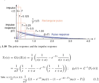
be applied to the system. Then the output gT(t), called the pulse response, is

(35)

1.2 Systems 19

Impulse

Impulse response

0 0.0

1

T=0.5

T=1.00

T rT(t)

gT(t)

Rectangular pulse

Pulse response

1.0 2.0 3.0 4.0 t

δ(t)

g(t)

0←T

T=0.125

T = 0.25

Fig. 1.10 The pulse response and the impulse response

YT(s)=G(s)X(s)=

1

T

₁

s(s+a) −e

−T s 1

s(s+a)

= 1 aT

1

s −

1

s+a −e

−T s

1

s −

1

s+a

; gT(t)=L−1{YT(s)}

Table A.1(3),(5),A.2(2)

= 1

aT

(1−e−at)us(t)−(1−e−a(t−T))us(t−T)

(1.2.17)

If we letT → 0 so that the rectangular pulse input becomes an impulseδ(t) (of instantaneous duration and infinite height), how can the output be expressed? Tak-ing the limit of the output equation (1.2.17) withT → 0, we can get the impulse responseg(t) (see Fig. 1.10):

gT(t) T→0

→ 1

aT

(1−e−at)us(t)−(1−e−a(t−T))us(t)

= 1 aT(e

aT₋

1)e−atus(t)

(D.25) ∼ =

aT→0 1

aT(1+aT−1)e

−at_u

s(t)=e−atus(t)

(1.2.14)

≡ g(t) (1.2.18)

This implies that as the input gets close to an impulse, the output becomes close to the impulse response, which is quite natural for any linear time-invariant system.

On the other hand, Fig. 1.11 shows the validity of Eq. (1.2.4) insisting that the linear combination of scaled/shifted pulse responses gets closer to the true output as

T →0.

1.2.6 Sinusoidal Steady-State Response

and Frequency Response

(36)

: x(t) : x(t)

: x(t) 1

0.5

0.5 1 1.5 2

0.4

0.2

0

0 1 2 3 4

0.4

0.2

0

0 1 2 3 4

0 1

0

1

0.5

0.5 1 1.5 2 0

0 ^

: x(t^ )

:y(t) = 2 3 1 2 3 4 5 1 2 3 5

1 2 3

4 3 2 1 T T + + +... :y(t) = 1+ +2 3

: y(t)

: y(t) (a1) The input x(t) and its approximation x^(t) with T = 0.5

(a2) The input x (t) and its approximation x^(t) with T = 0.25 (b2) The outputs to x(t) and x^(t) ^

(b1) The outputs to x(t) and x^(t)

^

Fig. 1.11 The input–output relationship of a linear time–invariant (LTI) system – convolution

response can be obtained from the time-domain input-output relationship (1.2.4). That is, noting that the sinusoidal input can be written as the sum of two complex conjugate exponential functions

x(t)= Acos (ωt+φ)(D=.21)A

2(e

j(ωt+φ)₊_e−j(ωt+φ)

)= A

2(x1(t)+x2(t)), (1.2.19) we substitutex1(t)=ej(ωt+φ)forx(t) into Eq. (1.2.4) to obtain a partial steady-state response as

y1(t)=G{x1(t)} (1.2.4)

=

∞

−∞

x1(τ)g(t−τ)dτ =

∞

−∞

ej(ωτ+φ)g(t−τ)dτ

=ej(ωt+φ)

∞

−∞

e−jω(t−τ)g(t−τ)dτ =ej(ωt+φ)

∞

−∞

e−jωtg(t)dt

=ej(ωt+φ)G(jω) (1.2.20)

with

G(jω)=

∞

−∞

e−jωtg(t)dtg(t)=0 for= t<0 causal system

∞

0

g(t)e−jωtdt(A=.1)G(s)|s=jω (1.2.21)

(37)

1.2 Systems 21

The total sinusoidal steady-state response to the sinusoidal input (1.2.19) can be expressed as the sum of two complex conjugate terms:

y(t)= A

2

y1(t)+y2(t)

= A

2

ej(ωt+φ)G(jω)+e−j(ωt+φ)G(−jω)

= A

2

ej(ωt+φ)|G(jω)|ejθ(ω)+e−j(ωt+φ)|G(−jω)|e−jθ(ω)

= A

2|G(jω)|

ej(ωt+φ+θ(ω))+e−j(ωt+φ+θ(ω))

(D.21)

= A|G(jω)|cos(ωt+φ+θ(ω)) (1.2.22)

where|G(jω)|andθ(ω)=∠G(jω) are the magnitude and phase of thefrequency response G(jω), respectively. Comparing this steady-state response with the sinu-soidal input (1.2.19), we see that its amplitude is|G(jω)|times the amplitudeAof the input and its phase isθ(ω) plus the phaseφof the input at the frequencyωof the input signal.

(cf.) The system function G(s) (Eq. (1.2.13a)) and frequency response G(jω) (Eq. (1.2.21)) of a system are the Laplace transform and Fourier transform of the impulse responseg(t) of the system, respectively.

Likewise, the sinusoidal steady-state response of a discrete-time system to a sinusoidal input, say,x[n]= Acos(Ωn+φ) turns out to be

y[n]= A|G[ejΩ]|cos(Ωn+φ+θ(Ω)) (1.2.23) where

G[ejΩ]=∞

n=−∞g[n]e

−jΩn g[n]=0 for₌ n<0

causal system

∞

n=0g[n]e

−jΩnRemark 4₌ .5

G[z]|_z₌_ejΩ

(1.2.24) Here we have used the definition (4.1) of thez-transform. Note thatG[ejΩ_{] obtained} by substitutingz=ejΩ₍_Ω_{: the digital frequency of the input signal) into the system} functionG[z] is called thefrequency response.

Remark 1.4Frequency Response and Sinusoidal Steady-State Response

(38)

(2) The steady-state response of a system to a sinusoidal input is also a sinusoidal signal of the same frequency. Its amplitude is the amplitude of the input times the magnitude of the frequency response at the frequency of the input. Its phase is the phase of the input plus the phase of the frequency response at the frequency of the input (see Fig. 1.12).

Input x(t) = Output y(t) = A⎪G(jω)⎪cos(ωt + φ + θ) : Magnitude of the frequency response : Phase of the frequency response

(a) A continuous-time system A cos(ωt + φ)

G(jω) θ(ω) = ∠G(jω)

G(s) Input x[n] = G[z] Output y[n] =

A⎪G(ejΩ₎_⎪cos(_Ω_{n + φ + θ}

)

(b) A discrete-time system A cos(Ωn + φ)

G[ejΩ

] : Magnitude of the frequency response θ(Ω) = ∠G[ejΩ

] : Phase of the frequency response

Fig. 1.12 The sinusoidal steady–state response of continuous-time/discrete-time linear time-invariant systems

1.2.7 Continuous/Discrete-Time Convolution

In Sect. 1.2.3, the output of an LTI system was found to be the convolution of the input and the impulse response. In this section, we take a look at the process of computing the convolution to comprehend its physical meaning and to be able to program the convolution process.

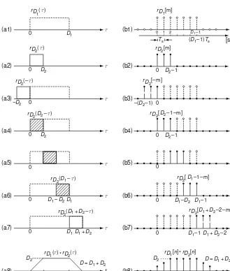
The continuous-time/discrete-time convolution y(t)/y[n] of two functions/ sequencesx(τ)/x[m] andg(τ)/g[m] can be obtained by time-reversing one of them, say,g(τ)/g[m] and time-shifting (sliding) it byt/ntog(t−τ)/g[n−m], multiplying it with the other, say,x(τ)/x[m], and then integrating/summing the multiplication, say,x(τ)g(t−τ)/x[m]g[n−m]. Let us take a look at an example.

Example 1.1Continuous-Time/Discrete-Time Convolution of Two Rectangular Pulses

(a) Continuous-Time Convolution (Integral) of Two Rectangular Pulse Functions

rD1(t) and rD2(t) Referring to Fig. 1.13(a1–a8), you can realize that the convolution of the two rectangular pulse functionsrD1(t) (of duration D1) and

rD2(t) (of durationD2 <D1) is

rD1(t)∗rD2(t)= ⎧ ⎪ ⎪ ⎪ ⎨

⎪ ⎪ ⎪ ⎩

t for 0≤t<D2

D2 forD2≤t <D1

−t+D forD1≤t <D=D1+D2

0 elsewhere

(E1.1.1a)

The procedure of computing this convolution is as follows:

- (a1) and (a2) showrD1(τ) andrD2(τ), respectively.

- (a3) shows the time-reversed version ofrD2(τ), that isrD2(−τ). Since there is no overlap betweenrD1(τ) andrD2(−τ), the value of the convolutionrD1(t)∗

(39)

1.2 Systems 23 (a1) (a2) (a3) (a4) (a5) (a6) (a7) (a8) D₂ D₂ –D₂ D₂ D₁ D₂ D₁ D₁ 0 0 0 0 0 0 0 0 D₁ D D=D₁ + D₂ r_D

1(τ)*rD2(τ) r_D

2(D1 – τ)

r_D

2(D1 + D2 – τ) r_D

2(D2 – τ) r_D

2(– τ) r_D

2( τ) r_D

1( τ)

t D₁ + D₂ D₁–D₂

τ (b1) (b2) (b3) (b4) (b5) (b6) (b7) (b8) 0 0 0 0 0 0

D=D₁ + D₂–1 r_D

1[n]*rD2[n]

D₂–1 D1–1

D₁–1 D2–1

–(D₂–1) 0 0 1 2

D₂–1

(D₁–1)T_s

D₁–1D–1 D₂

D1 + D2–2 r_D

2[D1 + D2–2–m] r_D

2[ D1–1–m] r_D

2[ D2–1–m] r_D

2[– m] r_D 2[m] r_D 1[m] m m m m m m m n D₁–D₂

T_s _[sec]τ

τ τ τ τ τ τ

D1–1

Fig. 1.13 Continuous–time/discrete–time convolution of two rectangular pulses

- (a4) shows the D2-delayed version ofrD2(−τ), that isrD2(D2−τ). Since this overlaps withrD1(τ) for 0≤τ <D2and the multiplication of them is 1 over the overlapping interval, the integration (area) isD2, which will be the value of the convolution att = D2. In the meantime (fromt =0 to D2), it gradually increases fromt =0 to