Maximal Overlap Discrete Wavelet Transform, Graph Theory And Backpropagation Neural Network In Stock Market Forecasting

(1)

41 IJNMT, Vol. V, No. 1 | June 2018

ISSN 2355-0082

Maximal Overlap Discrete Wavelet

Transform, Graph Theory And

Backpropagation Neural Network In Stock

Market Forecasting

Rosalina

1

_{, Hendra Jayanto}

2

Faculty of Computing, President University, Bekasi, Indonesia rosalina@president.ac.id

Received on November 23rd_{, 2017}

Accepted on June 8th_{, 2018}

Abstract—The aim of this paper is to get high accuracy of

stock market forecasting in order to produce signals that will affect the decision making in the trading itself. Several experiments by using different methodologies have been performed to answer the stock market forecasting issues. A traditional linear model, like autoregressive integrated moving average (ARIMA) has been used, but the result is not satisfactory because it is not suitable for model financial series. Yet experts are likely observed another approach by using artificial neural networks. Artificial neural network (ANN) are found to be more effective in realizing the input-output mapping and could estimate any continuous function which given an arbitrarily desired accuracy. In details, in this paper will use maximal overlap discrete wavelet transform (MODWT) and graph theory to distinguish and determine between low and high frequencies, which in this case acted as fundamental and technical prediction of stock market trading. After processed dataset is formed, then we will advance to the next level of the training process to generate the final result that is the buy or sell signals given from information whether the stock price will go up or down.

Index Terms—stock market, forecasting, maximal

overlap wavelet transform, artificial neural network, graph theory, backpropagation

I. INTRODUCTION

Forecasting stock market has been a hot topic in the last decades. It has been investigated, researched and experimented by researchers and professionals. A large number of methods for computing and stock predictions have been performed to solve the challenges [1]. The main issues of the forecasting are that the flow of the stocks hard to follow due to high volatility clustering and chaotic properties of stock market prices.

Several experiments by using different methodologies have been performed to answer the stock market forecasting issues. A traditional linear model, like autoregressive integrated moving average (ARIMA) has been used, but the results are not satisfactory because it is not suited to model financial

series. Yet experts are likely observing another approach by using artificial neural networks. Artificial neural network (ANN) are found effective in realizing the input-output mapping and can estimate any continuous function which given an arbitrarily desired accuracy. One of the ANN model proposed is back propagation algorithm (BP) [2], however this model also met two obstacles like low convergence rate and instability. On the other hand, another method yet to be observed is multi resolution analysis techniques like wavelet transform. It would likely give an unusual effects performed by wavelet processed data on the performance of numerical algorithms used to train the back-propagation algorithm.

The purpose of this paper is to aim for a high accuracy of stock market forecasting in order to produce signals that will affect the decision making in the trading itself. The paper is likely will combine several methods experimented before by another researchers to give processed data from raw data to be trained by artificial neural networks method. In details, we will use Maximal Overlap Discrete Wavelet Transform (MODWT) and graph theory to distinguish and determine between low and high frequencies, which in this case acted as fundamental and technical prediction of stock market trading. After processed dataset is formed, then we will advance to the next level of the training process to generate the final result that is the buy or sell signals given from information whether the stock price will go up or down. While the main contributions of this paper are:

 Combining MODWT and Graph theory in the preprocessing stage to extract stock features by using low and high frequencies as the representation of short and long term trend.

(2)

IJNMT, Vol. V, No. 1 | June 2018 42

ISSN 2355-0082

II. RELATED WORKS

Stock prediction is one of the most important issues in finance, various techniques have been adopted by researcher to predict the stock price.

Maximal Overlap Discrete Wavelet Transform have been implemented for decomposing the financial time series data [2,6,5,8,9] and to examine the effectiveness of high-frequency coefficients obtained from wavelet transforms in the prediction of stock prices, artificial neural networks (NN) were adopted [1,3,4].

Various kinds of wavelets are available such as the Haar,Mexican Hat, Morlet and Daubechies Wavelets [7]. In this paper, the Moving Average Discrete Wavelet Transform (MODWT) method were applied to decomposed the original signal.

III. METHODOLOGY

First of all the data collection will be conducted from online website, then the data will be processed through the attributes selection. Then after the attributes selection the data will be placed under wavelet transform to extract the features of the data. The next step that will be done is process the extracted features with the graph theory to get the strong correlation to give another attribute to the datasets. The last method is to train the complete datasets of training and test them with the testing datasets.

Figure 1. Methodology

1. Data Collection. Data Collection is the process of gathering and measuring information on variables of interest, in an established systematic fashion that enables one to answer stated research questions, test hypotheses, and evaluate outcomes. The goal for all data collection is to capture quality evidence that then translates to rich data analysis and allows the building of a convincing and credible answer to questions that have been posed.

The first step in this research is the data collection. In this stage, we carefully choose what types of data set will be used for the experiments.

The data of the stock market are varies and it contains a lot of types, there are Composite Index, Blue Chip stocks, and also common stocks. Besides that the other thing that we have to be concerned about is the marketplace itself, like American, European, and Asian, and other markets.

In these experiments the data sets collection selected is combination of Composite Index and Asian market. The main reason of the selection is that because the volatility of stock price movement for the Composite Index in Asian market is relatively stable so that will reduced the error possibilities produced.

We collect the data of Indonesian Stock Market Exchange (code: JKSE) from the online website. The data will conduct data from January 2010 until March 2015.

Table 1. The Data of Indonesian Stock Market Exchange

Date Open High Low Close Volume

Apr 16, 2014 4,883.49 4,893.54 4,870.61 4,873.01 4,263,442,400 Apr 15, 2014 4,872.30 4,893.23 4,863.01 4,870.21 4,069,120,000

The data contained variables of daily Date, Open, Close, Volume, Low, and High Prices can be seen in Table 2.

Table 1. Data Row Attributes

Name Description

Open Price when market open

Close Price when market close

Volume Stock market volume traded

High Price when market reach the highest of the day

Low Price when market reach the lowest of the day

Date Time when the stock market movement occurred

(3)

ISSN 2355-0082

constructed from the given one. For example in this experiment we add V_conv, δ , dim1, dim2, and dim3 to support the training and testing data set for the forecasting of stock market price. From the data pre-processing procedures we understand that the selection of attributes is depended on how the attributes affect the outcome of the model. In this case the main attributes (Open, Close, Volume, High, Low and Date) are still not sufficient to give the expected results outcome. Hence the dataset will be transformed into another form which will be used in the next stage (Date, Open, Close, V_conv, and δ(%)). Where we can get the attribute δ,

𝛿(%) =𝐶𝑙𝑜𝑠𝑒 − 𝑂𝑝𝑒𝑛_{𝑂𝑝𝑒𝑛} ∗ 100

Another attribute that we attained is the Volume Converted (𝑉_{𝑐𝑜𝑛𝑣}), where 𝑉_{𝑐𝑜𝑛𝑣}= 𝑉𝑜𝑙𝑢𝑚𝑒 for positive values of 𝛿(%) and 𝑉𝑐𝑜𝑛𝑣= −(𝑉𝑜𝑙𝑢𝑚𝑒) for negative values of 𝛿(%).

3. Wavelet Transform. Wavelet is a wave with amplitude begins at zero, increases and then decreases back to zero. Wavelet is very powerful for signal processing because it is constructed to have specific properties.

In this experiment, the wavelet transform used is Moving Average Discrete Wavelet Transform (MODWT). The using of this wavelet because MODWT is a wavelet transform algorithm that could overcome the lack of translation-invariance of discrete wavelet transforms.

The mother wavelet used is Daub4. The Haar wavelet has the advantage of very good time localization but the frequency resolution is minimal and not smooth. From the Haar wavelet we can see that the wavelet transform is equivalent to a filtering process with two filters, which divide the time series into wavelet part, which extracts the detail and the smoothed part. Daubechies discovered other filter coefficients. The simplest set has only 4 coefficients which famously known as Daub4. The selection of Daub4 is because it can extract the detail and the smoothed part, which cannot be done by Haar.

The datasets used for the training data and testing data are 2^n (to be precised 1024 dataset for training data and 32 set for testing).

The goal of this wavelet transform is to extract the features from the Open price and transform them into dimensions (dim), which then will be used for additional attributes for the final data set.

4. Graph Theory Correlation. The applicability of the graph theory is in determining of the three most significant attributes from MODWT dimensions. The three attributes attained by giving threshold for every wavelet dimension data set by observing the minimum and maximum value of every dimension and δ from the data set. After receiving the three significant dimensions referred as dim1, dim2, and dim3 we then proceed to the next stage.

5. Neural Network Training Model. In this neural network training we will train datasets from the training datasets supervisedly to be compared then with the testing datasets. The training datasets consists of several attributes like Open, Target (Close), 𝛿, 𝑉_𝑐𝑜𝑛, dim1, dim2 and dim3.

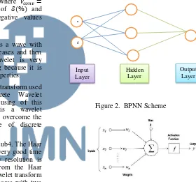
Figure 2. BPNN Scheme

Figure 3. Activation Function Scheme

For the neural network training that will be used is back propagation. The back propagation neural networks are feed-forward neural networks with one of more hidden layers that capable of approximating any continuous function up to certain accuracy with only one hidden layer. BPNN consists of three layers, named input layer (used to correspond to the problem’s input variable), hidden layer (used to capture the non-linear relationships among the variables) and output layer (used to provide the predicted values). Relationship between the output y(t) and the input x(t) is given:

𝑦(𝑡) = 𝑤(0) + ∑ 𝑤(𝑗)

𝑢

𝑗=1

. 𝑓 (𝑤(0, 𝑗) + ∑ 𝑤(𝑖, 𝑗). 𝑥(𝑡)

𝑣

𝑖=1

) n

d

Input Layer

Hidden Layer

Output Layer

(4)

ISSN 2355-0082

Activation Function scheme can be seen in Figure 3 with the activation functions for the output layer used are the sigmoid and hyperbolic functions. The objective function to minimize is the sum of the squares of the differences between the desirable output 𝑦𝑑(𝑡) and the predicted output 𝑦𝑝(𝑡). The training of that determines the length of the weight update, and m is the momentum parameter that allows escaping from small local minimal on the error surface and avoids having oscillations reduce the sensitivity of the network to fast changes in the error surface.

The parameter for the neural network is that training cycles 10000 epoch, learning rate 0.2, momentum 0.3, and error epsilon 10-5_.

Figure 4. Training Model Flowchart

6. Testing Model. The testing of the model is by comparing the data results of the applied model of backpropagation’s prediction results with the original data. The experiments consist of several kinds of data testing combination, using full portion of the same data with the training data, partial portion, and completely new data. using Backpropagation Neural Network (BPNN) for the forecasting.

Figure 5. Testing Model Flowchart

IV. RESEARCH RESULT

A. Experiment with JKSE (Asian Market Composite

Index)

The data used for the datasets are Indonesian stock exchange (JKSE) data vary from 2010 until 2015. To be exact, 1024 datasets will be used for the training and 32 datasets for the testing.

1. Data collection and Pre-processing. Since the data used for the dataset is data series then data JKSE from range 2010 until 2015 are collected. The select of JKSE data is because the JKSE movements are relatively stable with approximate changes 0.026%.

Figure 6. JKSE 2010 – 2015

Total dataset that will be used are 1024 in total for the training data and 32 dataset for testing. For the testing, here will be 3 scenarios:

a. Full training dataset

In this scenario all the dataset used are taken from the training set. In total there are 32 dataset used which exactly the same from the training dataset. It is expected that the accuracy of the forecasting will be high because there are already data template and target given for the testing data.

b. Half training and new dataset

For this second scenario, 32 dataset will be used for the testing which is half of the data (50%) taken from the training data and half others are new dataset. From this scenario it is expected that there would be dataset where all the dataset used are completely new which never computed in the training experiment before. From this experiment it is expected that although the accuracy from this experiment may be less than other two previous experiments, it still give out a good result, which still have high accuracy and better than experiments worked with any other methods ever.

1. MODWT and Graph Theory Data Collection

Begin Raw _Data Data Pre-processing

Date, Open,

Begin Raw _Data Data Pre-processing

(5)

ISSN 2355-0082

From the data processing then the experiment moved to process MODWT and Graph Theory. In this stage 1024 training dataset and 32 testing dataset will be conducted. The processing is using Open, Close, V_conv, and δ(%) variables which furthermore the Open variable is gone through normalization with threshold between -1 to 1. The results from the MODWT and graph theory led to the dimensions, dataset output, and attributes (Dim1, Dim2 Dim3) as shown in Table 3.

Table 3. Training and Testing Dataset

No. Results Training Dataset

Testing Dataset 1 Dimensions 11

Dimensions of low and high frequencies

6 Dimensions of low and high frequencies

2 Dataset output 1024 dataset 32 dataset

3 Dim1 (compatibility)

99.8% 69%

100% 63%

Table 4. Training Dataset for JKSE

Table 5. Testing Dataset for JKSE

2. Backpropagation

From the supervised training which using sigmoid activation, the results of the weight of every node in hidden layer by applying 10000 times training cycle (epoch). Several combinations of learning rate and momentum have been performed from 0.1 for the learning rate and 0.1 for the momentum until 0.9 for the learning rate and 0.9 for the momentum. The best combination for data learning is 0.1 and momentum 0.3. The result of the training model as follows in Table 5.

Table 5. BPNN Weighting Result

And for the output results also displayed as follows in

Table 6.

Table 6. Regression Result

In the visualization will be displayed as follow in Figure 7.

Figure 7. BPNN for JKSE Model

3. Final Results (accuracy and error)

(6)

ISSN 2355-0082

Table 7. Error Result of Enhanced MODWT– BPNN

Figure 8. Error Model Comparison for JKSE

From these experiments it is showed the results that by using DWT-BPNN the best result is by using full portion data of training set. This result is seemingly very possible because by using the exactly the same testing data with the training data, the pattern of the dataset is already determined so that resulting smaller error percentage in testing stage. The error for the real testing data (completely new data) is 43.75%, which is about 9.37% higher than the training-testing data’s error, which is 34.38%.

On the other side of the model applied by using MODWT, Graph theory and BPNN resulting that the error percentage conducted by using full portion training data as the testing data is the smallest, which showed 18.75%. It is not much differ in number with the experiment by using the full portion new dataset, which give error percentage about 18.8%. This diversity occurred by only 0.5% higher for the new testing dataset. The anomaly occurred in half portion data training set which in this case gave the largest error percentage, which showed 28.18%.

From this experiment by using JKSE dataset, it showed that in all testing dataset MODWT-Graph-BPNN performed better than DWT-MODWT-Graph-BPNN.

V. CONCLUSION

The results of this experiment stated that there are several major attributes that are significant to the computation of the model, such as Open, Target, V_conv, δ, dim1, dim2, and dim3.

It is also stated that the model of combined Enhanced MODWT-BPNN performed well for the JKSE stock index and performed best when the testing datasets are all new datasets. It performed less error than if the new dataset are combined with existing (training) datasets which the error showed 28.18% for combined datasets and 18.8% for the pure new datasets.

REFERENCES

[1] Adebiyi, A., Ayo, C., Adebiyi, M. , Otokiti, S., Stock Price Prediction using Neural Network with Hybridized Market Indicators, 2012

[2] Caetano, M.A.L., Yoneyama, T., Forecasting Short Term Abrupt Changes in the Stock Market with Wavelet Decomposition and Graph Theory, 2012

[3] G. Zhang, B.E. Patuwo, M.Y. Hu, Forecasting with artificial neural networks: the state of the art, Int. J. Forecast., 14, pp. 35-62, 1998,

[4] G.S. Atsalakis, K.P. Valavanis, Surveying stock market forecasting techniques – Part II: soft computing methods,Expert Syst. Appl., 36, pp. 5932-5941, 2009 [5] Lahmiri, S., Wavelet Low- and High-Frequency Components

as Features for Predicting Stock Prices with Backpropagation Neural Networks, 2014

[6] Liu, H., Chen, C., Tian, H., & Li, Y.,A hybrid model for wind speed prediction using empirical mode decomposition and artificial neural networks. Renewable Energy, 2012 [7] R.M. Rao, A.S. Bopardikar, Wavelet Transforms: Introduction

to Theory and Applications, Addison Wesley, Boston, 1998 [8] S.-C. Huang, T.-K. Wu, Integrating recurrent SOM with

wavelet-based kernel partial least square regressions for financial forecasting, Expert Syst. Appl., 37, pp. 5698-5705, 2010