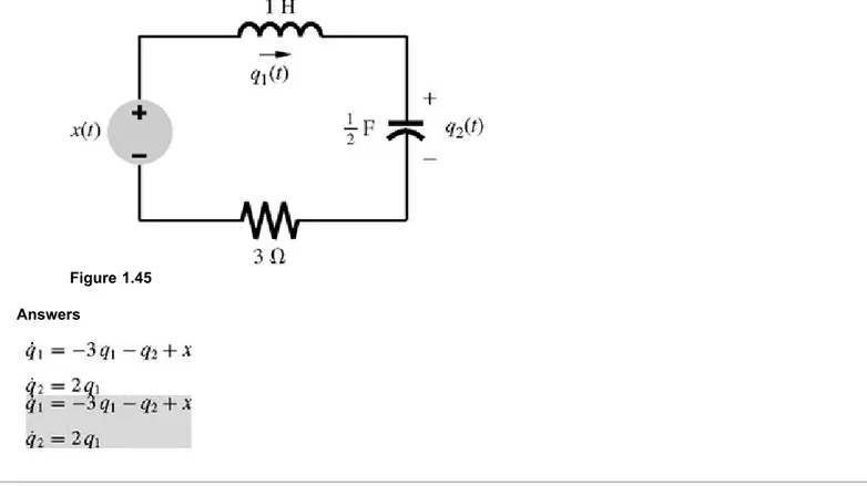
Linear Systems and Signals, Second Edition
B. P. LathiOxford University Press 2005
Published by Oxford University Press, Inc.
198 Madison Avenue, New York, New York 10016 http://www.oup.com
© 2005 Oxford University Press, Inc.
Oxford is a registered trademark of Oxford University Press
All rights reserved. No part of this publication may be reproduced, stored in a retrieval system, or transmitted, in any form or by any means, electronic, mechanical, photocopying, recording, or otherwise, without the prior permission of Oxford University Press.
1. Signal processing—Mathematics. 2. System analysis. 3. Linear time invariant systems. 4. Digital filters (Mathematics) I. Title.
TK5102.5L298 2004
621.382′2—dc22 2003064978
9 8 7 6 5 4 3 2 1
Preface
This book, Linear Systems and Signals, presents a comprehensive treatment of signals and linear systems at an introductory level. Like all my other books, it emphasizes physical appreciation of concepts through heuristic reasoning, and the use of metaphors, analogies, and creative explanations. Such an approach is much different from a purely deductive technique that uses mere mathematical manipulation of symbols. There is a temptation to treat engineering subjects as a branch of applied mathematics. Such an approach is a perfect match to the public image of engineering as a dry and dull discipline. It ignores the physical meaning behind various derivations and deprives a student of intuitive grasp and the enjoyable experience of logical uncovering of the subject matter. Here I have used mathematics not so much to prove axiomatic theory as to support and enhance physical and intuitive understanding. Wherever possible, theoretical results are interpreted heuristically and are enhanced by carefully chosen examples and analogies.
This second edition, which closely follows the organization of the first edition, has been refined by incorporating suggestions and changes provided by various reviewers. The added topics include Bode plots, use of digital filters in an impulse-invariance method of designing analog systems, convergence of infinite series, bandpass systems, group and phase delay, and Fourier applications to communication systems. A significant and sizable addition in the area of MATLAB® (a registered trademark of The Math Works, Inc.) has been provided by Dr. Roger Green of North Dakota State University. Dr. Green discusses his contribution at the conclusion of this preface.
ORGANIZATION
The book may be conceived as divided into five parts:
1. Introduction (Background and Chapter 1).
2. Time-domain analysis of linear time-invariant (LTI) systems (Chapters 2 and 3).
3. Frequency-domain (transform) analysis of LTI systems (Chapters 4 and 5).
5. State-space analysis of LTI systems (Chapter 10).
The organization of the book permits much flexibility in teaching the continuous-time and discrete-time concepts. The natural sequence of chapters is meant to integrate continuous-time and discrete-time analysis. It is also possible to use a sequential approach in which all the continuous-time analysis is covered first (Chapters 1, 2, 4, 6, 7, and 8), followed by discrete-time analysis (Chapters 3, 5, and 9).
SUGGESTIONS FOR USING THIS BOOK
The book can be readily tailored for a variety of courses spanning 30 to 45 lecture hours. Most of the material in the first eight chapters can be covered at a brisk pace in about 45 hours. The book can also be used for a 30-lecture-hour course by covering only analog material (Chapters 1, 2, 4, 6, 7, and possibly selected topics in Chapter 8). Alternately, one can also select Chapters 1 to 5 for courses purely devoted to systems analysis or transform techniques. To treat continuous- and discrete-time systems by using an integrated (or parallel) approach, the appropriate sequence of Chapters is 1, 2, 3, 4, 5, 6, 7, and 8. For a sequential approach, where the continuous-time analysis is followed by discrete-time analysis, the proper chapter sequence is 1, 2, 4, 6, 7, 8, 3, 5, and possibly 9 (depending on the time availability).
Logically, the Fourier transform should precede the Laplace transform. I have used such an approach in the companion
volume, Signal Processing and Linear Systems (Oxford, 1998). However, a sizable number of instructors feel that it is easier for students to learn Fourier after Laplace. Such an approach has an appeal because of the gradual progression of difficulty, in the sense that the relatively more difficult concepts of Fourier are treated after the simpler area of Laplace. This book is written to accommodate that viewpoint. For those who wish to see Fourier before Laplace, there is Signal Processing and Linear Systems.
NOTABLE FEATURES
The notable features of this book include the following:
1. Intuitive and heuristic understanding of the concepts and physical meaning of mathematical results are
emphasized throughout. Such an approach not only leads to deeper appreciation and easier comprehension of the concepts, but also makes learning enjoyable for students.
2. Many students are handicapped by an inadequate background in basic material such as complex numbers, sinusoids, quick sketching of functions, Cramer's rule, partial fraction expansion, and matrix algebra. I have added a chapter that addresses these basic and pervasive topics in electrical engineering. Response by students has been unanimously enthusiastic.
3. There are more than 200 worked examples in addition to exercises (usually with answers) for students to test their understanding. There is also a large number of selected problems of varying difficulty at the end of each chapter.
4. For instructors who like to get students involved with computers, several examples are worked out by means of MATLAB, which is becoming a standard software package in electrical engineering curricula. There is also a MATLAB session at the end of each chapter. The problem set contains several computer problems. Working computer examples or problems, though not essential for the use of this book, is highly recommended.
5. The discrete-time and continuous-time systems may be treated in sequence, or they may be integrated by using a parallel approach.
6. The summary at the end of each chapter proves helpful to students in summing up essential developments in the chapter.
7. There are several historical notes to enhance student's interest in the subject. This information introduces students to the historical background that influenced the development of electrical engineering.
ACKNOWLEDGMENTS
Several individuals have helped me in the preparation of this book. I am grateful for the helpful suggestions of the several reviewers. I am most grateful to Prof. Yannis Tsividis of Columbia University, who provided his comprehensively thorough and insightful feedback for the book. I also appreciate another comprehensive review by Prof. Roger Green. I thank Profs. Joe Anderson of Tennessee Technological University, Kai S. Yeung of the University of Texas at Arlington, and Alexander
Arizona, and William Edward Pierson from the U.S. Air Force Research Laboratory. Only those who write a book understand that writing a book such as this is an obsessively time-consuming activity, which causes much hardship for the family members, where the wife suffers the most. So what can I say except to thank my wife, Rajani, for enormous but invisible sacrifices.
B. P. Lathi
MATLAB
MATLAB is a sophisticated language that serves as a powerful tool to better understand a myriad of topics, including control theory, filter design, and, of course, linear systems and signals. MATLAB's flexible programming structure promotes rapid development and analysis. Outstanding visualization capabilities provide unique insight into system behavior and signal character. By exploring concepts with MATLAB, you will substantially increase your comfort with and understanding of course topics.
As with any language, learning MATLAB is incremental and requires practice. This book provides two levels of exposure to MATLAB. First, short computer examples are interspersed throughout the text to reinforce concepts and perform various computations. These examples utilize standard MATLAB functions as well as functions from the control system, signal processing, and symbolic math toolboxes. MATLAB has many more toolboxes available, but these three are commonly available in many engineering departments.
A second and deeper level of exposure to MATLAB is achieved by concluding each chapter with a separate MATLAB session. Taken together, these eleven sessions provide a self-contained introduction to the MATLAB environment that allows even novice users to quickly gain MATLAB proficiency and competence. These sessions provide detailed instruction on how to use MATLAB to solve problems in linear systems and signals. Except for the very last chapter, special care has been taken to avoid the use of toolbox functions in the MATLAB sessions. Rather, readers are shown the process of developing their own code. In this way, those readers without toolbox access are not at a disadvantage.
All computer code is available online (http://www.mathworks.com/support/books). Code for the computer examples in a given chapter, say Chapter xx, is named CExx.m. Program yy from MATLAB Session xx is named MSxxPyy.m. Additionally, complete code for each individual MATLAB session is named MSxx.m.
Chapter B:
Background
The topics discussed in this chapter are not entirely new to students taking this course. You have already studied many of these topics in earlier courses or are expected to know them from your previous training. Even so, this background material deserves a review because it is so pervasive in the area of signals and systems. Investing a little time in such a review will pay big dividends later. Furthermore, this material is useful not only for this course but also for several courses that follow. It will also be helpful later, as reference material in your professional career.
B.1 COMPLEX NUMBERS
Complex numbers are an extension of ordinary numbers and are an integral part of the modern number system. Complex numbers, particularly imaginary numbers, sometimes seem mysterious and unreal. This feeling of unreality derives from their unfamiliarity and novelty rather than their supposed nonexistence! Mathematicians blundered in calling these numbers "imaginary," for the term immediately prejudices perception. Had these numbers been called by some other name, they would have become demystified long ago, just as irrational numbers or negative numbers were. Many futile attempts have been made to ascribe some physical meaning to imaginary numbers. However, this effort is needless. In mathematics we assign symbols and operations any meaning we wish as long as internal consistency is maintained. The history of mathematics is full of entities that were unfamiliar and held in abhorrence until familiarity made them acceptable. This fact will become clear from the following historical note.
B.1-1 A Historical Note
Among early people the number system consisted only of natural numbers (positive integers) needed to express the number of children, cattle, and quivers of arrows. These people had no need for fractions. Whoever heard of two and one-half children or three and one-fourth cows!
However, with the advent of agriculture, people needed to measure continuously varying quantities, such as the length of a field and the weight of a quantity of butter. The number system, therefore, was extended to include fractions. The ancient Egyptians and Babylonians knew how to handle fractions, but Pythagoras discovered that some numbers (like the diagonal of a unit square) could not be expressed as a whole number or a fraction. Pythagoras, a number mystic, who regarded numbers as the essence and principle of all things in the universe, was so appalled at his discovery that he swore his followers to secrecy and imposed a death penalty for divulging this secret.[1] These numbers, however, were included in the number system by the time of Descartes, and they are now known as irrational numbers.
Until recently, negative numbers were not a part of the number system. The concept of negative numbers must have appeared absurd to early man. However, the medieval Hindus had a clear understanding of the significance of positive and negative numbers.[2], [3] They were also the first to recognize the existence of absolute negative quantities.[4] The works of Bhaskar (1114-1185) on arithmetic (Līlāvatī) and algebra (Bījaganit) not only use the decimal system but also give rules for dealing with negative quantities. Bhaskar recognized that positive numbers have two square roots.[5] Much later, in Europe, the men who developed the banking system that arose in Florence and Venice during the late Renaissance (fifteenth century) are credited with introducing a crude form of negative numbers. The seemingly absurd subtraction of 7 from 5 seemed reasonable when bankers began to allow their clients to draw seven gold ducats while their deposit stood at five. All that was necessary for this purpose was to write the difference, 2, on the debit side of a ledger.[6]
Thus the number system was once again broadened (generalized) to include negative numbers. The acceptance of negative numbers made it possible to solve equations such as x + 5 = 0, which had no solution before. Yet for equations such as x2 + 1 = 0, leading to x2 = −1, the solution could not be found in the real number system. It was therefore necessary to define a completely new kind of number with its square equal to −1. During the time of Descartes and Newton, imaginary (or complex) numbers came to be accepted as part of the number system, but they were still regarded as algebraic fiction. The Swiss mathematician Leonhard Euler introduced the notation i (for imaginary) around 1777 to represent √−1. Electrical engineers use the notation j instead of i to avoid confusion with the notation i often used for electrical current. Thus
and
This notation allows us to determine the square root of any negative number. For example,
When imaginary numbers are included in the number system, the resulting numbers are called complex numbers.
ORIGINS OF COMPLEX NUMBERS
Ironically (and contrary to popular belief), it was not the solution of a quadratic equation, such as x2 + 1 = 0, but a cubic equation with real roots that made imaginary numbers plausible and acceptable to early mathematicians. They could dismiss √−1 as pure nonsense when it appeared as a solution to x2 + 1 = 0 because this equation has no real solution. But in 1545, Gerolamo Cardano of Milan published Ars Magna (The Great Art), the most important algebraic work of the Renaissance. In this book he gave a method of solving a general cubic equation in which a root of a negative number appeared in an intermediate step. According to his method, the solution to a third-order equation[†]
Gerolamo Cardano
For example, to find a solution of x3 + 6x− 20 = 0, we substitute a = 6, b = −20 in the foregoing equation to obtain
We can readily verify that 2 is indeed a solution of x3 + 6x− 20 = 0. But when Cardano tried to solve the equation x3− 15x− 4 = 0 by this formula, his solution was
What was Cardano to make of this equation in the year 1545? In those days negative numbers were themselves suspect, and a square root of a negative number was doubly preposterous! Today we know that
Therefore, Cardano's formula gives
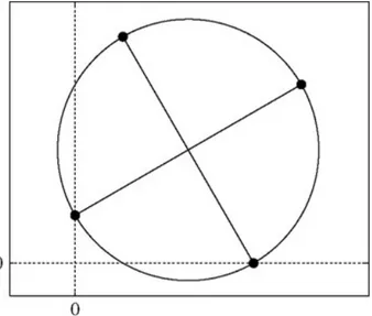
We can readily verify that x = 4 is indeed a solution of x3− 15x− 4 = 0. Cardano tried to explain halfheartedly the presence of but ultimately dismissed the whole enterprize as being "as subtle as it is useless." A generation later, however, Raphael Bombelli (1526-1573), after examining Cardano's results, proposed acceptance of imaginary numbers as a necessary vehicle that would transport the mathematician from the real cubic equation to its real solution. In other words, although we begin and end with real numbers, we seem compelled to move into an unfamiliar world of imaginaries to complete our journey. To mathematicians of the day, this proposal seemed incredibly strange.7 Yet they could not dismiss the idea of imaginary numbers so easily because this concept yielded the real solution of an equation. It took two more centuries for the full importance of complex numbers to become evident in the works of Euler, Gauss, and Cauchy. Still, Bombelli deserves credit for recognizing that such numbers have a role to play in algebra.7
In 1799 the German mathematician Karl Friedrich Gauss, at the ripe age of 22, proved the fundamental theorem of algebra, namely that every algebraic equation in one unknown has a root in the form of a complex number. He showed that every equation of the nth order has exactly n solutions (roots), no more and no less. Gauss was also one of the first to give a coherent account of complex numbers and to interpret them as points in a complex plane. It is he who introduced the term "complex numbers" and paved the way for their general and systematic use. The number system was once again broadened or generalized to include imaginary numbers. Ordinary (or real) numbers became a special case of generalized (or complex) numbers.
Figure B.1: Use of complex numbers can reduce the work.
B.1-2 Algebra of Complex Numbers
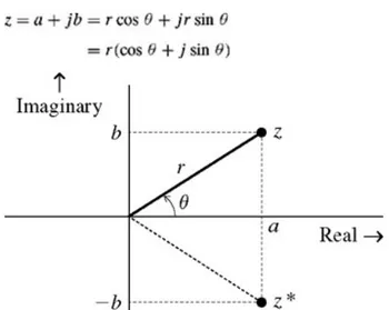
A complex number (a, b) or a + jb can be represented graphically by a point whose Cartesian coordinates are (a, b) in a complex plane (Fig. B.2). Let us denote this complex number by z so that
The numbers a and b (the abscissa and the ordinate) of z are the real part and the imaginary part, respectively, of z. They are also expressed as
Note that in this plane all real numbers lie on the horizontal axis, and all imaginary numbers lie on the vertical axis.
Complex numbers may also be expressed in terms of polar coordinates. If (r, θ) are the polar coordinates of a point z = a + jb (see Fig. B.2), then
and
Figure B.2: Representation of a number in the complex plane. The Euler formula states that
Hence, it follows that[†]
Using Eq. (B.3) in (B.2) yields
Thus, a complex number can be expressed in Cartesian form a + jb or polar form rejθ with
and
Observe that r is the distance of the point z from the origin. For this reason, r is also called the magnitude (or absolute value) of z and is denoted by |z|. Similarly, θ is called the angle of z and is denoted by ∠z. Therefore
and
Also
CONJUGATE OF A COMPLEX NUMBER We define z*, the conjugate of z = a + jb, as
The graphical representation of a number z and its conjugate z* is depicted in Fig. B.2. Observe that z* is a mirror image of z about the horizontal axis. To find the conjugate of any number, we need only replace j by −j in that number (which is the same as changing the sign of its angle). The sum of a complex number and its conjugate is a real number equal to twice the real part of the number:
The product of a complex number z and its conjugate is a real number |z|2, the square of the magnitude of the number:
UNDERSTANDING SOME USEFUL IDENTITIES
Figure B.3: Understanding some useful identities in terms of rejθ. In fact,
The number 1, on the other hand, is also at a unit distance from the origin, but has an angle 2π (in fact, ±2nπ for any integer value of n). Therefore,
The number j is at unit distance from the origin and its angle is π/2 (see Fig. B.3b). Therefore,
Similarly,
Thus
In fact,
This discussion shows the usefulness of the graphic picture of rej. This picture is also helpful in several other applications. For example, to determine the limit of e(α+jw)t as t→∞, we note that
Now the magnitude of ejwt is unity regardless of the value of ω or t because ejwt = rejθ with r = 1. Therefore, eαt determines the behavior of e(α+jω)t as t→∞ and
In future discussions you will find it very useful to remember rejθ as a number at a distance r from the origin and at an angle θ with the horizontal axis of the complex plane.
A WARNING ABOUT USING ELECTRONIC CALCULATORS IN COMPUTING ANGLES
From the Cartesian form a + jb we can readily compute the polar form rejθ [see Eq. (B.6)]. Electronic calculators provide ready conversion of rectangular into polar and vice versa. However, if a calculator computes an angle of a complex number by using an inverse trigonometric function θ = tan−1 (b/a), proper attention must be paid to the quadrant in which the number is located. For instance, θ corresponding to the number −2 −j3 is tan−1 (−3/−2). This result is not the same as tan−1 (3/2). The former is −123.7°, whereas the latter is 56.3°. An electronic calculator cannot make this distinction and can give a correct answer only for angles in the first and fourth quadrants. It will read tan−1(−3/−2) as tan−1 (3/2), which is clearly wrong. When you are computing inverse trigonometric functions, if the angle appears in the second or third quadrant, the answer of the calculator is off by 180°. The correct answer is obtained by adding or subtracting 180° to the value found with the calculator (either adding or subtracting yields the correct answer). For this reason it is advisable to draw the point in the complex plane and determine the quadrant in which the point lies. This issue will be clarified by the following examples.
EXAMPLE B.1
Express the following numbers in polar form: a. 2 + j3
b. −2 + j3 c. −2 −j3 d. 1 −j3
a.
write
b.
Figure B.4: From Cartesian to polar form.
In this case the angle is in the second quadrant (see Fig. B.4b), and therefore the answer given by the calculator, tan−1 (1/−2) =
−26.6°, is off by 180°. The correct answer is (−26.6 ± 180)° = 153.4° or −206.6°. Both values are correct because they represent the same angle.
It is a common practice to choose an angle whose numerical value is less than 180°. Such a value is called the principal value of the angle, which in this case is 153.4°. Therefore,
c.
In this case the angle appears in the third quadrant (see Fig. B.4c), and therefore the answer obtained by the calculator (tan−1 (−3/−2) = 56.3°) is off by 180°. The correct answer is (56.3° 180)° = 236.3° or −123.7°. We choose the principal value −123.7° so that (see
Fig. B.4c).
d.
In this case the angle appears in the fourth quadrant (see Fig. B.4d), and therefore the answer given by the calculator, tan−1 (−3/1) =
−71.6°, is correct (see Fig. B.4d):
COMPUTER EXAMPLE CB.1
Using the MATLAB function cart2pol, convert the following numbers from Cartesian form to polar form: a. z = 2 + j3
b. z = −2 + j1
b. Therefore, z = 2 + j3 = 3.6056ej0.98279 + 3.6056ej56.3099°
Therefore, z = −2 + j1 = 2.2361ej2.6779 = 2.2361ej153.4349°. >> [z_rad, z_mag] = cart2pol(2, 3); >> z_deg = z_rad* (180/pi);
>> disp(['(a) z_mag = ',num2str(z_mag),'; z_rad = ',num2str(z_rad), ... >> '; z_deg = ',num2str(z_deg)]);
(a) z mag = 3.6056; z rad = 0.98279; z deg = 56.3099
>> [z_rad, z_mag] = cart2pol(-2, 1); >> z_deg = z_rad* (180/pi);
>> disp(['(b) z_mag = ',num2str(z_mag),'; z_rad = ',num2str(z_rad), ... >> '; z_deg = ',num2str(z_deg)]);
EXAMPLE B.2
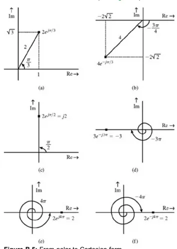
Represent the following numbers in the complex plane and express them in Cartesian form: a. 2ejπ/3
b. 4e−j3π/4 c. 2ejπ/2 d. 3e−j3π e. 2ej4π
f. 2e−j4π
a. 2ejπ/3 = 2(cos π/3 + j sin π/3) = 1 + j√3 (See Fig. B.5b)
Figure B.5: From polar to Cartesian form.
b. 4e−j3π/4 = 4(cos 3π/4 −j sin π/4) = −2√2 −j2 √2 (See Fig. B.5b) c. 2ejπ/2 = 2(cos π/2 + j sin π/2) = 2(0 + j 1) = j2 (See Fig. B.5c) d. 3e−j3π = 2(cos 3π−j sin 3π) = 3(−1 + j0) = −3 (See Fig. B.5d) e. 2ej4π = 2(cos 4π + j sin 4π) = 2(1 −j0) = 2 (See Fig. B.5e)
f. 2e−j4π = 2(cos 4π−j sin 4π) = 2(1 −j0) = 2 (See Fig. B.5f) COMPUTER EXAMPLE CB.2
Using the MATLAB function pol2cart, convert the number z = 4e−j(3π/4) from polar form to Cartesian form.
Therefore, z = 4e−j(3π/4) = −2.8284 −j2.8284.
ARITHMETICAL OPERATIONS, POWERS, AND ROOTS OF COMPLEX NUMBERS
To perform addition and subtraction, complex numbers should be expressed in Cartesian form. Thus, if >> [z_real, z_imag] = pol2cart(-3*pi/4,4);
and
then
If z1 and z2 are given in polar form, we would need to convert them into Cartesian form for the purpose of adding (or subtracting). Multiplication and division, however, can be carried out in either Cartesian or polar form, although the latter proves to be much more convenient. This is because if z1 and z2 are expressed in polar form as
then
and
Moreover,
and
This shows that the operations of multiplication, division, powers, and roots can be carried out with remarkable ease when the numbers are in polar form.
Strictly speaking, there are n values for z1/n (the nth root of z). To find all the n roots, we reexamine Eq. (B.15d).
The value of z1/n given in Eq. (B.15d) is the principal value of z1/n, obtained by taking the nth root of the principal value of z, which corresponds to the case k = 0 in Eq. (B.15e).
EXAMPLE B.3
Determine z1z2 and z1/z2 for the numbers
We shall solve this problem in both polar and Cartesian forms. MULTIPLICATION: CARTESIAN FORM
MULITPLICATION: POLAR FORM
DIVISION: CARTESIAN FORM
To eliminate the complex number in the denominator, we multiply both the numerator and the denominator of the right-hand side by 2 −j3, the denominator's conjugate. This yields
DIVISION: POLAR FORM
It is clear from this example that multiplication and division are easier to accomplish in polar form than in Cartesian form. EXAMPLE B.4
b. 1/z1 c. z1/z22
d.
a. Since subtraction cannot be performed directly in polar form, we convert z1 and z2 to Cartesian form:
Therefore,
b.
c.
d. There are three cube roots of 8ej(π/3) = 8ejj(π/3+2k), k = 0, 1, 2.
The principal value (value corresponding to k = 0) is 2ejπ/9.
COMPUTER EXAMPLE CB.3
Determine z1z2 and z1/z2 if z1 = 3 + j4 and z2 = 2 + j3
Therefore, z1z2 = (3 + j4)(2 + j3) = −6 + j17 and z1/z2 = (3 + j4)/(2 + j3) = 1.3486 −j0.076923. EXAMPLE B.5
Consider X(ω), a complex function of a real variable ω:
a. Express X(ω) in Cartesian form, and find its real and imaginary parts. b. Express X(ω) in polar form, and find its magnitude |X(ω)| and angle ∠X(ω).
a. To obtain the real and imaginary parts of X (ω), we must eliminate imaginary terms in the denominator of X (ω). This is readily done by multiplying both the numerator and the denominator of X(ω) by 3 −j4ω, the conjugate of the denominator 3 + j4ω so that
This is the Cartesian form of X(ω). Clearly the real and imaginary parts Xr(ω) and Xi(ω) are given by
b.
This is the polar representation of X(ω). Observe that >> z_1 = 3+j*4; z_2 = 2+j*3;
>> z_1z_2 = z_1*z_2; >> z_1divz_2 = z_1/z_2;
LOGARITHMS OF COMPLEX NUMBERS We have
if
then
The value of In z for k = 0 is called the principal value of In z and is denoted by Ln z.
In all these expressions, the case of k = 0 is the principal value of that expression. [1]Calinger, R., ed. Classics of Mathematics. Moore Publishing, Oak Park, IL, 1982. [2]Hogben, Lancelot. Mathematics in the Making. Doubleday, New York, 1960. [3]Cajori, Florian. A History of Mathematics, 4th ed. Chelsea, New York, 1985. [4]Encyclopaedia Britannica. Micropaedia IV, 15th ed., vol. 11, p. 1043. Chicago, 1982.
[5]Singh, Jagjit. Great Ideas of Modern Mathematics. Dover, New York, 1959. [6]Dunham, William. Journey Through Genius. Wiley, New York, 1990.
[†]This equation is known as the depressed cubic equation. A general cubic equation
can always be reduced to a depressed cubic form by substituting y = x− (p/3). Therefore any general cubic equation can be solved if we know the solution to the depressed cubic. The depressed cubic was independently solved, first by Scipione del Ferro (1465-1526) and then by Niccolo Fontana (1499-1557). The latter is better known in the history of mathematics as Tartaglia ("Stammerer"). Cardano learned the secret of the depressed cubic solution from Tartaglia. He then showed that by using the substitution y = x− (p/3), a general cubic is reduced to a depressed cubic.
[†]It can be shown that when we impose the following three desirable properties on an exponential ez where z = x + jy, we come to conclusion that
ejy = cos y + j sin y (Euler equation). These properties are 1. ez is a single-valued and analytic function of z. 2. dez/dz = ez
3. ez reduces to ex if y = 0.
We know that
Therefore, cos φ repeats itself for every change of 2π in the angle φ. For the sinusoid in Eq. (B.18), the angle 2πf0t + θ changes by 2π when t changes by 1/f0. Clearly, this sinusoid repeats every 1/f0 seconds. As a result, there are f0 repetitions per second. This is the frequency of the sinusoid, and the repetition interval T0 given by
is the period. For the sinusoid in Eq. (B.18), C is the amplitude, f0 is the frequency (in hertz), and θ is the phase. Let us consider two special cases of this sinusoid when θ = 0 and θ = −π/2 as follows:
a. x(t) = C cos 2πf0t (θ = 0)
b. x(t) = C cos (2πf0t−π/2) = C sin 2πf0t (θ = −π/2)
The angle or phase can be expressed in units of degrees or radians. Although the radian is the proper unit, in this book we shall often use the degree unit because students generally have a better feel for the relative magnitudes of angles expressed in degrees rather than in radians. For example, we relate better to the angle 24° than to 0.419 radian. Remember, however, when in doubt, use the radian unit and, above all, be consistent. In other words, in a given problem or an expression do not mix the two units.
It is convenient to use the variable ω0 (radian frequency) to express 2π/f0:
With this notation, the sinusoid in Eq. (B.18) can be expressed as
in which the period T0 is given by [see Eqs. (B.19) and (B.20)]
and
In future discussions, we shall often refer to ω0 as the frequency of the signal cos (ω0t + θ), but it should be clearly understood that the frequency of this sinusoid is f0 Hz (f0 = ω0/2π), and ω0 is actually the radian frequency.
Figure B.6: Sketching a sinusoid.
This signal can be obtained by shifting (delaying) the signal C cos ω0t (Fig. B.6a) to the right by a phase (angle) of 60°. We know that a sinusoid undergoes a 360° change of phase (or angle) in one cycle. A quarter-cycle segment corresponds to a 90° change of angle. We therefore shift (delay) the signal in Fig. B.6a by two-thirds of a quarter-cycle segment to obtain C cos (ω0t− 60°), as shown in Fig. B.6c.
Observe that if we delay C cos ω0t in Fig. B.6a by a quarter-cycle (angle of 90° or π/2 radians), we obtain the signal C sin ω0t, depicted in Fig. B.6b. This verifies the well-known trigonometric identity
Alternatively, if we advance C sin ω0t by a quarter-cycle, we obtain C cos ω0t. Therefore,
This observation means sin ω0t lags cos ω0t by 90°(π/2 radians), or cos ω0t leads sin ω0t by 90°.
B.2-1 Addition of Sinusoids
Two sinusoids having the same frequency but different phases add to form a single sinusoid of the same frequency. This fact is readily seen from the well-known trigonometric identity
in which
Therefore,
Equations (B.23b) and (B.23c) show that C and θ are the magnitude and angle, respectively, of a complex number a−jb. In other words, a−jb = Cejθ. Hence, to find C and θ, we convert a−jb to polar form and the magnitude and the angle of the resulting polar number are C and θ, respectively.
To summarize,
in which C and θ are given by Eqs. (B.23b) and (B.23c), respectively. These happen to be the magnitude and angle, respectively, of a−jb. The process of adding two sinusoids with the same frequency can be clarified by using phasors to represent sinusoids. We represent the sinusoid C cos (ω0t + θ) by a phasor of length C at an angle θ with the horizontal axis. Clearly, the sinusoid a cos ω0t is represented by a horizontal phasor of length a (θ = 0), while b sin ω0t = b cos (ω0t−π/2) is represented by a vertical phasor of length b at an angle −π/2 with the horizontal (Fig. B.7). Adding these two phasors results in a phasor of length C at an angle θ, as depicted in Fig. B.7. From this figure, we verify the values of C and θ
found in Eqs. (B.23b) and (B.23c), respectively.
Figure B.7: Phasor addition of sinusoids.
Proper care should be exercised in computing θ, as explained on page 8 ("A Warning About Using Electronic Calculators in Computing Angles"). EXAMPLE B.6
In the following cases, express x(t) as a single sinusoid: a. x(t) = cos ω0t−√3 sin ω0t
a. In this case, a = 1, b = −√3, and from Eqs. (B.23)
Therefore,
We can verify this result by drawing phasors corresponding to the two sinusoids. The sinusoid cos ω0t is represented by a phasor of unit length at a zero angle with the horizontal. The phasor sin ω0t is represented by a unit phasor at an angle of −90° with the
horizontal, Therefore, −√3 sin ω0t is represented by a phasor of length √2 at 90° with the horizontal, as depicted in Fig. B.8a. The two phasors added yield a phasor of length 2 at 60° with the horizontal (also shown in Fig. B.8a).
Figure B.8: Phasor addition of sinusoids.
Alternately, we note that a−jb = 1 + j√3 = 2ejπ/3. Hence, C = 2 and θ = π/3.
Observe that a phase shift of ±π amounts to multiplication by −1. Therefore, x(t) can also be expressed alternatively as
In practice, the principal value, that, is, −120°, is preferred. b. In this case, a = −3, b = 4, and from Eqs. (B.23) we have
Observe that
Therefore,
This result is readily verified in the phasor diagram in Fig. B.8b. Alternately, a−jb = −3 −j4 = 5e−j126.9°. Hence, C = 5 and θ =
−126.9°. COMPUTER EXAMPLE CB.4
Express f(t) = −3 cos (ω0t) + 4 sin (ω0t) as a single sinusoid.
Notice that a cos (ω0t) + b sin (ω0t) = C cos [ω0t + tan−1 (−b/a)]. Hence, the amplitude C and the angle θ of the resulting sinusoid are the magnitude and angle of a complex number a − jb.
Therefore, f(t) = −3 cos (ω0t) + 4 sin (ω0t) = 5 cos (ω0t− 2.2143) = 5 cos (ω0t− 126.8699°). We can also perform the reverse operation, expressing
in terms of cos ω0t and sin ω0t by means of the trigonometric identity >> a= -3; b = 4;
>> [theta,C] = cart2pol(a,-b); >> theta_deg = (180/pi)*theta;
>> disp(['C = ',num2str(C),'; theta = ',num2str(theta),... >> '; theta_deg = ',nu,2str(theta_deg)]);
For example,
B.2-2 Sinusoids in Terms of Exponentials: Euler's Formula
Sinusoids can be expressed in terms of exponentials by using Euler's formula [see Eq. (B.3)]
Inversion of these equations yields
B.3 SKETCHING SIGNALS
In this section we discuss the sketching of a few useful signals, starting with exponentials.
B.3-1 Monotonic Exponentials
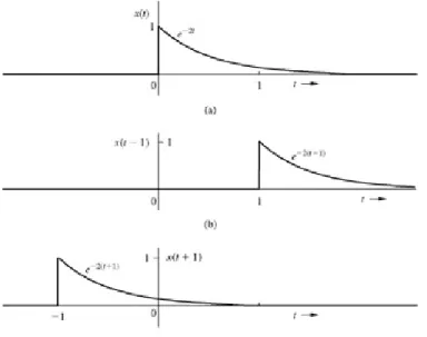
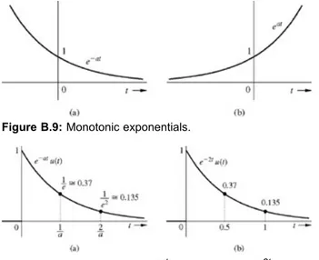
The signal e−at decays monotonically, and the signal eat grows monotonically with t (assuming a > 0) as depicted in Fig. B.9. For the sake of simplicity, we shall consider an exponential e−at starting at t = 0, as shown in Fig. B.10a.
Figure B.9: Monotonic exponentials.
Figure B.10: (a) Sketching e−at. (b) Sketching e−2t.
The signal e−at has a unit value at t = 0. At t = 1/a, the value drops to 1/e (about 37% of its initial value), as illustrated in Fig. B.10a. This time interval over which the exponential reduces by a factor e (i.e., drops to about 37% of its value) is known as the time constant of the exponential. Therefore, the time constant of e−at is 1/a. Observe that the exponential is reduced to 37% of its initial value over any time interval of duration 1/a. This can be shown by considering any set of instants t1 and t2 separated by one time constant so that
Now the ratio of e−at2 to e−at1 is given by
We can use this fact to sketch an exponential quickly. For example, consider
The time constant in this case is 0.5. The value of x(t) at t = 0 is 1. At t = 0.5 (one time constant) it is 1/e (about 0.37). The value of x(t) continues to drop further by the factor 1/e (37%) over the next half-second interval (one time constant). Thus x(t) at t = 1 is (1/e)2. Continuing in this manner, we see that x(t) = (1/e)3 at t = 1.5, and so on. A knowledge of the values of x(t) at t = 0, 0.5, 1, and 1.5 allows us to sketch the desired signal as shown in Fig. B.10b.[†]
B.3-2 The Exponentially Varying Sinusoid
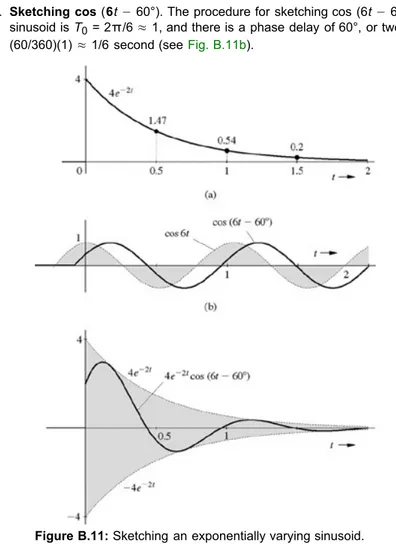
We now discuss sketching an exponentially varying sinusoidLet us consider a specific example:
We shall sketch 4e−2t and cos (6t− 60°) separately and then multiply them:
i. Sketching 4e−2t. This monotonically decaying exponential has a time constant of 0.5 second and an initial value of 4 at t = 0.
Therefore, its values at t = 0.5, 1, 1.5, and 2 are 4/e, 4/e2, 4/e3, and 4/e4, or about 1.47, 0.54, 0.2, and 0.07, respectively. Using these values as a guide, we sketch 4e−2t, as illustrated in Fig. B.11a.
ii. Sketching cos (6t− 60°). The procedure for sketching cos (6t− 60°) is discussed in Section B.2 (Fig. B.6c). Here the period of the sinusoid is T0 = 2π/6 ≈ 1, and there is a phase delay of 60°, or two-thirds of a quarter-cycle, which is equivalent to a delay of about (60/360)(1) ≈ 1/6 second (see Fig. B.11b).
Figure B.11: Sketching an exponentially varying sinusoid.
iii. Sketching 4e−2t cos (6t− 60°). We now multiply the waveforms in steps i and ii. This multiplication amounts to forcing the sinusoid 4 cos (6t− 60°) to decrease exponentially with a time constant of 0.5. The initial amplitude (at t = 0) is 4, decreasing to 4/e (= 1.47) at t = 0.5, to 1.47/e (= 0.54) at t = 1, and so on. This is depicted in Fig. B.11c. Note that when cos (6t− 60°) has a value of unity (peak amplitude),
Therefore, 4e−2t cos (6t− 60°) touches 4e−2t at the instants at which the sinusoid cos (6t− 60°) is at its positive peaks. Clearly 4e−2t is an envelope for positive amplitudes of4e−2t cos (6t− 60°). Similar argument shows that 4e−2t cos (6t− 60°) touches −4e−2t at its negative peaks. Therefore, −4e−2t is an envelope for negative amplitudes of 4e−2t cos (6t− 60°). Thus, to sketch 4e−2t cos (6t− 60°), we first draw the envelopes 4e−2t and −4e−2t (the mirror image of 4e−2t about the horizontal axis), and then sketch the sinusoid cos (6t− 60°), with these envelopes acting as constraints on the sinusoid's amplitude (see Fig. B.11c).
In general, Ke−at cos (ω0t + θ) can be sketched in this manner, with Ke−at and −Ke−at constraining the amplitude of cos (ω0t + θ).
B.4 CRAMER'S RULE
Cramer's rule offers a very convenient way to solve simultaneous linear equations. Consider a set of n linear simultaneous equations in n unknowns x1, x2,..., xn:
These equations can be expressed in matrix form as
We denote the matrix on the left-hand side formed by the elements aij as A. The determinant of A is denoted by |A|. If the determinant |A| is not
zero, the set of equations (B.29) has a unique solution given by Cramer's formula
where |Dk| is obtained by replacing the kth column of |A| by the column on the right-hand side of Eq. (B.30) (with elements y1, y2,..., yn). We shall demonstrate the use of this rule with an example.
EXAMPLE B.7
Use Cramer's rule to solve the following simultaneous linear equations in three unknowns:
In matrix form these equations can be expressed as
Here,
Since |A| = 4 ≠ 0, a unique solution exists for x1, x2, and x3. This solution is provided by Cramer's rule [Eq. (B.31)] as follows:
B.5 PARTIAL FRACTION EXPANSION
The function F(x) is improper if m≧n and proper if m < n. An improper function can always be separated into the sum of a polynomial in x and a proper function. Consider, for example, the function
Because this is an improper function, we divide the numerator by the denominator until the remainder has a lower degree than the denominator.
Therefore, F(x) can be expressed as
A proper function can be further expanded into partial fractions. The remaining discussion in this section is concerned with various ways of doing this.
B.5-1 Method of Clearing Fractions
A rational function can be written as a sum of appropriate partial fractions with unknown coefficients, which are determined by clearing fractions and equating the coefficients of similar powers on the two sides. This procedure is demonstrated by the following example.
EXAMPLE B.8
Expand the following rational function F(x) into partial fractions:
This function can be expressed as a sum of partial fractions with denominators (x + 1), (x + 2), (x + 3), and (x + 3)2, as follows:
To determine the unknowns k1, k2, k3, and k4 we clear fractions by multiplying both sides by (x + 1)(x + 2)(x + 3)2 to obtain
Equating coefficients of similar powers on both sides yields
Solution of these four simultaneous equations yields
Therefore,
Although this method is straightforward and applicable to all situations, it is not necessarily the most efficient. We now discuss other methods that can reduce numerical work considerably.
Distinct Factors Of Q(x)
We shall first consider the partial fraction expansion of F(x) = P(x)/Q(x), in which all the factors of Q(x) are distinct (not repeated). Consider the proper function
We can show that F(x) in Eq. (B.35a) can be expressed as the sum of partial fractions
To determine the coefficient k1, we multiply both sides of Eq. (B.35b) by x−λ1 and then let x = λ1. This yields
On the right-hand side, all the terms except k1 vanish. Therefore,
Similarly, we can show that
This procedure also goes under the name method of residues.
EXAMPLE B.9
Expand the following rational function F(x) into partial fractions:
To determine k1, we let x = −1 in (x + 1) F(x). Note that (x + 1)F(x) is obtained from F(x) by omitting the term (x + 1) from its denominator. Therefore, to compute k1 corresponding to the factor (x + 1), we cover up the term (x + 1) in the denominator of F(x) and then substitute x = −1 in the remaining expression. [Mentally conceal the term (x + 1) in F(x) with a finger and then let x = −1 in the remaining expression.] The steps in covering up the function
are as follows.
Step 1. Cover up (conceal) the factor (x + 1) from F(x):
Step 2. Substitute x = −1 in the remaining expression to obtain k1:
Similarly, to compute k2, we cover up the factor (x− 2) in F(x) and let x = 2 in the remaining function, as follows:
and
Therefore,
Complex Factors Of Q(x)
where
Similarly,
Therefore,
The coefficients k2 and k3 corresponding to the complex conjugate factors are also conjugates of each other. This is generally true when the coefficients of a rational function are real. In such a case, we need to compute only one of the coefficients.
Quadratic Factors
Often we are required to combine the two terms arising from complex conjugate factors into one quadratic factor. For example, F(x) in Eq. (B.38) can be expressed as
The coefficient k1 is found by the Heaviside method to be 2. Therefore,
The values of c1 and c2 are determined by clearing fractions and equating the coefficients of similar powers of x on both sides of the resulting equation. Clearing fractions on both sides of
Eq. (B.40) yields
Equating terms of similar powers yields c1 = 2, c2 = −8, and
SHORTCUTS
The values of c1 and c2 in Eq. (B.40) can also be determined by using shortcuts. After computing k1 = 2 by the Heaviside method as before, we let
x = 0 on both sides of Eq. (B.40) to eliminate c1. This gives us
Therefore,
To determine c1, we multiply both sides of Eq. (B.40) by x and then let x→∞. Remember that when x→∞, only the terms of the highest power are significant. Therefore,
and
other convenient values for x, such as x = 1. Consider the case
We find k = 1 by the Heaviside method in the usual manner. As a result,
To determine c1 and c2, if we try letting x = 0 in Eq. (B.43), we obtain ∞ on both sides. So let us choose x = 1. This yields
or
We can now choose some other value for x, such as x = 2, to obtain one more relationship to use in determining c1 and c2. In this case, however, a simple method is to multiply both sides of Eq. (B.43) by x and then let x→∞. This yields
so that
Therefore,
B.5-3 Repeated Factors of
Q
(
x
)
If a function F(x) has a repeated factor in its denominator, it has the form
Its partial fraction expansion is given by
The coefficients k1, k2,..., kj corresponding to the unrepeated factors in this equation are determined by the Heaviside method, as before [Eq. (B.37)]. To find the coefficients a0, a1, a2,..., ar−1, we multiply both sides of Eq. (B.45) by (x−λ)r. This gives us
If we let x = λ on both sides of Eq. (B.46), we obtain
Therefore, a0 is obtained by concealing the factor (x−λ)r in F(x) and letting x = λ in the remaining expression (the Heaviside "cover-up" method). If we take the derivative (with respect to x) of both sides of Eq. (B.46), the right-hand side is a1 + terms containing a factor (x−λ) in their numerators. Letting x = λ on both sides of this equation, we obtain
Thus, a1 is obtained by concealing the factor (x−λ)r in F(x), taking the derivative of the remaining expression, and then letting x = λ. Continuing in this manner, we find
Observe that (x−λ)rF(x) is obtained from F(x) by omitting the factor (x−λ)r from its denominator. Therefore, the coefficient aj is obtained by
EXAMPLE B.10
Expand F(x) into partial fractions if
The partial fractions are
The coefficient k is obtained by concealing the factor (x + 2) in F(x) and then substituting x = −2 in the remaining expression:
To find a0, we conceal the factor (x + 1)3 in F(x) and let x = −1 in the remaining expression:
To find a1, we conceal the factor (x + 1)3 in F(x), take the derivative of the remaining expression, and then let x = −1:
Similarly,
Therefore,
B.5-4 Mixture of the Heaviside "Cover-Up" and Clearing Fractions
For multiple roots, especially of higher order, the Heaviside expansion method, which requires repeated differentiation, can become cumbersome. For a function that contains several repeated and unrepeated roots, a hybrid of the two procedures proves to be the best. The simpler coefficients are determined by the Heaviside method, and the remaining coefficients are found by clearing fractions or shortcuts, thus incorporating the best of the two methods. We demonstrate this procedure by solving Example B.10 once again by this method.
In Example B.10, coefficients k and a0 are relatively simple to determine by the Heaviside expansion method. These values were found to be k1 = 1 and a0 = 2. Therefore,
We now multiply both sides of this equation by (x + 1)3 (x + 2) to clear the fractions. This yields
Equating coefficients of the third and second powers of x on both sides, we obtain
We may stop here if we wish because the two desired coefficients, a1 and a2, are now determined. However, equating the coefficients of the two remaining powers of x yields a convenient check on the answer. Equating the coefficients of the x1 and x0 terms, we obtain
These equations are satisfied by the values a1 = 1 and a2 = 3, found earlier, providing an additional check for our answers. Therefore,
which agrees with the earlier result.
In Example B.10, after determining the coefficients a0 = 2 and k = 1 by the Heaviside method as before, we have
There are only two unknown coefficients, a1 and a2. If we multiply both sides of this equation by x and then let x→∞, we can eliminate a1. This yields
Therefore,
There is now only one unknown a1, which can be readily found by setting x equal to any convenient value, say x = 0. This yields
which agrees with our earlier answer.
There are other possible shortcuts. For example, we can compute a0 (coefficient of the highest power of the repeated root), subtract this term from both sides, and then repeat the procedure.
B.5-5 Improper
F
(
x
) with
m
=
n
A general method of handling an improper function is indicated in the beginning of this section. However, for a special case of the numerator and denominator polynomials of F(x) being of the same degree (m = n), the procedure is the same as that for a proper function. We can show that for
the coefficients k1, k2,..., kn are computed as if F(x) were proper. Thus,
For quadratic or repeated factors, the appropriate procedures discussed in Sections B.5-2 or B.5-3 should be used as if F(x) were proper. In other words, when m = n, the only difference between the proper and improper case is the appearance of an extra constant bn in the latter. Otherwise the
procedure remains the same. The proof is left as an exercise for the reader. EXAMPLE B.11
Expand F(x) into partial fractions if
Here m = n = 2 with bn = b2 = 3. Therefore,
in which
and
Therefore,
B.5-6 Modified Partial Fractions
In finding the inverse z-transforms (Chapter 5), we require partial fractions of the form kx/(x−λi)r rather than k/(x−λi)r. This can be achieved by
Dividing both sides by x yields
Expansion of the right-hand side into partial fractions as usual yields
Using the procedure discussed earlier, we find a1 = 1, a2 = 1, a3 = −2, and a4 = 1. Therefore,
Now multiplying both sides by x yields
This expresses F(x) as the sum of partial fractions having the form kx/(x−λi)r.
B.6 VECTORS AND MATRICES
An entity specified by n numbers in a certain order (ordered n-tuple) is an n-dimensional vector. Thus, an ordered n-tuple (x1, x2,..., xn) represents
an n-dimensional vector x. A vector may be represented as a row (row vector):
or as a column (column vector):
Simultaneous linear equations can be viewed as the transformation of one vector into another. Consider, for example, the n simultaneous linear equations
If we define two column vectors x and y as
then Eqs. (B.48) may be viewed as the relationship or the function that transforms vector x into vector y. Such a transformation is called the linear transformation of vectors. To perform a linear transformation, we need to define the array of coefficients aij appearing in Eqs. (B.48). This array is
called a matrix and is denoted by A for convenience:
A matrix with m rows and n columns is called a matrix of the order (m, n) or an (m × n) matrix. For the special case of m = n, the matrix is called a square matrix of order n.
It should be stressed at this point that a matrix is not a number such as a determinant, but an array of numbers arranged in a particular order. It is convenient to abbreviate the representation of matrix A in Eq. (B.50) with the form (aij) m x n, implying a matrix of order m x n with aij as its ijth
element. In practice, when the order m x n is understood or need not be specified, the notation can be abbreviated to (aij). Note that the first index i
of aij indicates the row and the second index j indicates the column of the element aij in matrix A.
or
Equation (B.51) is the symbolic representation of Eq. (B.48). Yet we have not defined the operation of the multiplication of a matrix by a vector. The quantity Ax is not meaningful until such an operation has been defined.
B.6-1 Some Definitions and Properties
A square matrix whose elements are zero everywhere except on the main diagonal is a diagonal matrix. An example of a diagonal matrix is
A diagonal matrix with unity for all its diagonal elements is called an identity matrix or a unit matrix, denoted by I. This is a square matrix:
The order of the unit matrix is sometimes indicated by a subscript. Thus, In represents the n−n unit matrix (or identity matrix). However, we shall
omit the subscript. The order of the unit matrix will be understood from the context. A matrix having all its elements zero is a zero matrix.
A square matrix A is a symmetric matrix if aij = aij (symmetry about the main diagonal).
Two matrices of the same order are said to be equal if they are equal element by element. Thus, if
then A = B only if aij = bij for all i and j.
If the rows and columns of an m × n matrix A are interchanged so that the elements in the ith row now become the elements of the ith column (for i = 1, 2,..., m), the resulting matrix is called the transpose of A and is denoted by AT. It is evident that AT is an n x m matrix. For example, if
Thus, if
then
Note that
B.6-2 Matrix Algebra
We shall now define matrix operations, such as addition, subtraction, multiplication, and division of matrices. The definitions should be formulated so that they are useful in the manipulation of matrices.
ADDITION OF MATRICES
For two matrices A and B, both of the same order (m × n),
or
Note that two matrices can be added only if they are of the same order. MULTIPLICATION OF A MATRIX BY A SCALAR
We multiply a matrix A by a scalar c as follows:
We also observe that the scalar c and the matrix A commute, that is,
MATRIX MULTIPLICATION We define the product
in which cij, the element of C in the ith row and jth column, is found by adding the products of the elements of A in the ith row with the
corresponding elements of B in the jth column. Thus,
This result is expressed as follows:
Note carefully that if this procedure is to work, the number of columns of A must be equal to the number of rows of B. In other words, AB, the product of matrices A and B, is defined only if the number of columns of A is equal to the number of rows of B. If this condition is not satisfied, the product AB is not defined and is meaningless. When the number of columns of A is equal to the number of rows of B, matrix A is said to be conformable to matrix B for the product AB. Observe that if A is an m × n matrix and B is an n × p matrix, A and B are conformable for the product, and C is an m × p matrix.
We demonstrate the use of the rule in Eq. (B.56) with the following examples.
In both cases, the two matrices are conformable. However, if we interchange the order of the matrices as follows,
the matrices are no longer conformable for the product. It is evident that in general,
this is true, matrices A and B are said to commute. We reemphasize that in general, matrices do not commute.
In the matrix product AB, matrix A is said to be postmultiplied by B or matrix B is said to be premultiplied by A. We may also verify the following relationships:
We can verify that any matrix A premultiplied or postmultiplied by the identity matrix I remains unchanged:
Of course, we must make sure that the order of I is such that the matrices are conformable for the corresponding product. We give here, without proof, another important property of matrices:
where |A| and |B| represent determinants of matrices A and B. MULTIPLICATION OF A MATRIX BY A VECTOR
Consider the matrix Eq. (B.52), which represents Eq. (B.48). The right-hand side of Eq. (B.52) is a product of the m × n matrix A and a vector x. If, for the time being, we treat the vector x as if it were an n × 1 matrix, then the product Ax, according to the matrix multiplication rule, yields the right-hand side of Eq. (B.48). Thus, we may multiply a matrix by a vector by treating the vector as if it were an n × 1 matrix. Note that the constraint of conformability still applies. Thus, in this case, xA is not defined and is meaningless.
MATRIX INVERSION
To define the inverse of a matrix, let us consider the set of equations represented by Eq. (B.52):
We can solve this set of equations for x1,x2,...,xn in terms of y1, y2,..., yn, by using Cramer's rule [see Eq. (B.31)]. This yields
in which |A| is the determinant of the matrix A and |Dij| is the cofactor of element aij in the matrix A. The cofactor of element aij is given by (−1)i+j
times the determinant of the (n − 1) × (n − 1) matrix that is obtained when the ith row and the jth column in matrix A are deleted. We can express Eq. (B.62a) in matrix form as
We now define A−1, the inverse of a square matrix A, with the property
Then, premultiplying both sides of Eq. (B.63) by A−1, we obtain
or
A comparison of Eq. (B.65) with Eq. (B.62b) shows that
implies that the matrix A must be a square matrix. In addition, we observe from the solution as given in Eq. (B.62b) that if the solution is to exist, |A|
≠ 0.[†] Therefore, the inverse exists only for a square matrix and only under the condition that the determinant of the matrix be nonzero. A matrix whose determinant is nonzero is a nonsingular matrix. Thus, an inverse exists only for a nonsingular, square matrix. By definition, we have
Postmultiplying this equation by A−1 and then premultiplying by A, we can show that
Clearly, the matrices A and A−1 commute.
The operation of matrix division can be accomplished through matrix inversion. EXAMPLE B.12
Let us find A−1 if
Here
and |A| = −4. Therefore,
B.6-3 Derivatives and Integrals of a Matrix
Elements of a matrix need not be constants; they may be functions of a variable. For example, if
then the matrix elements are functions of t. Here, it is helpful to denote A by A(t). Also, it would be helpful to define the derivative and integral of A(t).
The derivative of a matrix A(t) (with respect to t) is defined as a matrix whose ijth element is the derivative (with respect to t) of the ijth element of the matrix A. Thus, if
then
or
Thus, the derivative of the matrix in Eq. (B.68) is given by
Similarly, we define the integral of A(t) (with respect to t) as a matrix whose ijth element is the integral (with respect to t) of the ijth element of the matrix A:
Thus, for the matrix A in Eq. (B.68), we have
The proofs of identities (B.71a) and (B.71b) are trivial. We can prove Eq. (B.71c) as follows. Let A be an m x n matrix and B an n x p matrix. Then, if
from Eq. (B.56), we have
and
or
Equation (B.72) along with the multiplication rule clearly indicate that dik is the ikth element of matrix and eik is the ikth element of matrix Equation (B.71c) then follows.
If we let B = A−1 in Eq. (B.71c), we obtain
But since
we have
B.6-4 The Characteristic Equation of a Matrix: The Cayley-Hamilton Theorem
For an (n − n) square matrix A, any vector x (x≠ 0) that satisfies the equationis an eigenvector (or characteristic vector), and λ is the corresponding eigenvalue (or characteristic value) of A.Equation (B.74) can be expressed as
The solution for this set of homogeneous equations exists if and only if
or
Equation (B.76a) [or (B.76b)] is known as the characteristic equation of the matrix A and can be expressed as
Q(λ) is called the characteristic polynomial of the matrix A. The n zeros of the characteristic polynomial are the eigenvalues of A and, corresponding to each eigenvalue, there is an eigenvector that satisfies Eq. (B.74).
FUNCTIONS OF A MATRIX
We now demonstrate the use of the Cayley-Hamilton theorem to evaluate functions of a square matrix A. Consider a function f(λ) in the form of an infinite power series:
Since λ, being an eigenvalue (characteristic root) of A, satisfies the characteristic equation [Eq. (B.77)], we can write
If we multiply both sides by λ, the left-hand side is λn+1, and the right-hand side contains the terms λn, λn-1, ..., λ. Using Eq. (B.80), we substitute
λn, in terms of λn−1, ?n-2,..., λ so that the highest power on the right-hand side is reduced to n− 1. Continuing in this way, we see that λn+k can
be expressed in terms of λn-1, ?n-2,...,λ for any k. Hence, the infinite series on the right-hand side of Eq. (B.79) can always be expressed in terms of
λn−1, λn−2,λ,λ and a constant as
If we assume that there are n distinct eigenvalues ?1, ?2,..., λn, then Eq. (B.81) holds for these n values of λ. The substitution of these values in Eq. (B.81) yields n simultaneous equations
and
Since A also satisfies Eq. (B.80), we may advance a similar argument to show that if f(A) is a function of a square matrix A expressed as an infinite power series in A, then
and, as argued earlier, the right-hand side can be expressed using terms of power less than or equal to n− 1,
in which the coefficients βis are found from Eq. (B.82b). If some of the eigenvalues are repeated (multiple roots), the results are somewhat modified.
We shall demonstrate the utility of this result with the following two examples.
B.6-5 Computation of an Exponential and a Power of a Matrix
Let us compute eAt defined byFrom Eq. (B.83b), we can express
in which the βis are given by Eq. (B.82b), with f(λi) = eλit. EXAMPLE B.13
The characteristic equation is
Hence, the eigenvalues are λ1 = −1, λ2 = −2, and
in which
and
COMPUTATION OF Ak
As Eq. (B.83b) indicates, we can express Ak as
in which the βis are given by Eq. (B.82b) with f(λi) = λki. For a completed example of the computation of Ak by this method, see Example 10.12. [†]These two conditions imply that the number of equations is equal to the number of unknowns and that all the equations are independent.
B.7 MISCELLANEOUS
B.7-1 L'Hôpital's Rule
If lim f(x)/g(x) results in the indeterministic form 0/0 or ∞/∞, then
B.7-2 The Taylor and Maclaurin Series
B.7-4 Sums
B.7-5 Complex Numbers
B.7-8 Common Derivative Formulas
B.7-10 Solution of Quadratic and Cubic Equations
Any quadratic equation can be reduced to the formThe solution of this equation is provided by
A general cubic equation
may be reduced to the depressed cubic form
by substituting
This yields
Now let
The solution of the depressed cubic is
and
REFERENCES
1. Asimov, Isaac. Asimov on Numbers. Bell Publishing, New York, 1982.
2. Calinger, R., ed. Classics of Mathematics. Moore Publishing, Oak Park, IL, 1982. 3. Hogben, Lancelot. Mathematics in the Making. Doubleday, New York, 1960. 4. Cajori, Florian. A History of Mathematics, 4th ed. Chelsea, New York, 1985. 5. Encyclopaedia Britannica. Micropaedia IV, 15th ed., vol. 11, p. 1043. Chicago, 1982. 6. Singh, Jagjit. Great Ideas of Modern Mathematics. Dover, New York, 1959.
7. Dunham, William. Journey Through Genius. Wiley, New York, 1990.
MATLAB SESSION B: ELEMENTARY OPERATIONS
MB.1 MATLAB OVERVIEW
Although MATLAB(r) (a registered trademark of The Math Works, Inc.) is easy to use, it can be intimidating to new users. Over the years, MATLAB has evolved into a sophisticated computational package with thousands of functions and thousands of pages of documentation. This section provides a brief introduction to the software environment.
When MATLAB is first launched, its command window appears. When MATLAB is ready to accept an instruction or input, a command prompt (>>) is displayed in the command window. Nearly all MATLAB activity is initiated at the command prompt.
![Figure MB.4: h α (t) for α = [0,1,..., 10].](https://thumb-ap.123doks.com/thumbv2/123dok/2757693.1681379/45.918.57.409.84.356/figure-mb-h-a-t-a.webp)