Long-term Peak Load Forecasting Using
LM-Feedforward Neural Network for Java-Madura-Bali
Interconnection, Indonesia
Yusak Tanoto*1, Weerakorn Ongsakul +, and Charles O.P. Marpaung +
Abstract – This paper presents the application of artificial neural network (ANN) based on multi-layered feedforward backpropagation for long-term peak load forecasting (LTPF). A four-layered network using Levenberg-Marquardt (LM) learning algorithm is proposed to forecast annual peak load of Java-Madura-Bali interconnection, Indonesia, for the period of 2009-2018 considering 11 regional factors encompass economic, electricity statistics, and weather thought to affect the load demand. The proposed network structure is first trained over the past 11 years (1995-2005) to forecast annual peak load of 2006-2008. Afterwards, the justified network structure is trained over the past 14 years (1995-2008) to forecast annual peak load of 2009-2018. Several simulations involve changes in historical actual peak load target and variation on projected regional economic growth are carried out to observe the network adaptability. Results are then compared with that achieved by the multiple regression model and projection made by utility. In this case, forecasting result exhibited by the proposed network is the closest to actual values of 2006-2009 among others taken the average error of 0.2%. Likewise, its forecasting differences for 2010-2018 are less than 7% compared to others. In term of network adaptability, outputs generated by the network are well adjusted to the projected inputs variation.
Keywords – Artificial neural network, Java-Madura-Bali interconnection, LM algorithm, long-term peak load forecasting.
1. INTRODUCTION
Annual peak load forecasting is substantial to meet long-term electricity demand appropriately through system planning and expansion. In the long run, LTPF is a prominent precondition to establish the national electricity policy with respect to energy resources utilization and the selection of appropriate energy technologies based on the least cost, taken into account the environmental issues.
Two general methods have been applied on LTPF are artificial inteligent (AI) and econometric. Over the decades, ANN has been extensively used on this area and it has reported satisfactory performance better than that achieved by econometric method [1]-[4]. ANN offers flexibility in applying the customized model in order to increase its capability of pattern mapping as well as to meet certain requirement.
In the case of Java-Madura-Bali interconnection (hereafter “JaMaLi”), Indonesia, a LTPF has been done using Feedforward network with variable learning rate algorithm for 2007-2025, taken into account 10 actual historical data of 2001-2006 [5]. However, there is no verification in term of the network performance in the absence of comparison between the network forecasting result and the corresponding actual peak load.
In this paper, a four-layered LM-feedforward structure is proposed for the case of JaMaLi taken into account 11 actual historical and projection factors in economic, electricity statistics, and weather during the
*
Electrical Engineering Department, Petra Christian University, Jl. Siwalankerto 121-131 Surabaya 60236, East Java, Indonesia.
+
Energy Field of Study, Asian Institute of Technology, P.O. Box 4, Klong Luang, Pathumthani 12120, Thailand.
E-mail: [email protected]; [email protected].
1
Corresponding author;
Tel: + 62 31 849 4830 ext 3445, Fax: + 62 31 841 7658
period of 1995-2018. Benefits of LM algorithm over variable learning rate and conjugate gradient method are reported in [6]. The overview of electricity sector in Indonesia, methodology, simulations and results, and conclusion are described further in the following sections.
2. OVERVIEW OF ELECTRICITY SECTOR IN
INDONESIA
The total national installed capacity of electricity supply until mid 2008 was 29,885 MW, of which the state-owned enterprise (hereafter “PLN”) contributed 24,924 MW or 83.39%, whereas private power generation companies contributed 4,044 MW or 13.53%, followed by captive power accounted for 916 MW or 3.08% [7]. In 2008, total installed capacity under the PLN system for JaMaLi was 18,538 MW, composed of 87.1% thermal power plants and 12.9% hydropower plants [8].
The total national electricity consumption was around 129,100 GWh, of which 128,810 GWh consumed through PLN system, where JaMaLi was accounted for 100,425 GWh. As per sector wise, industrial sector in JaMaLi was consumed the highest electricity accounted for 42,554 GWh, followed by residential sector with 35,929 GWh. However, the highest sectoral growth for 1995-2008 was attained by commercial sector as it has grown from 4,071.75 GWh to 16,947.63 GWh, or 316.2% [8]-[9].
3. METHODOLOGY
3.1 Network data set
Actual historical data over the past 14 years (1995-2008) are applied as an input vector to the network considering input consistency as several electricity statistics data prior 1995 are based on government fiscal calendar. The input variables with respect to JaMaLi are: (1) Gross Regional Domestic Product (GRDP) with adjusted deflator, (2) population, (3) number of households, (4) total electricity energy consumption, (5) total installed power contracted, (6-9) electricity energy consumption in residential sector, commercial sector, industrial sector, and public sector, (10) electrification ratio, and (11) cooling degree days (CDD). JaMaLi’s annual peak load during the same period are taken as the training output target.
In addition, the same 11 factors as it has been officially projected are assembled accordingly together with the JaMaLi’s annual peak load projection made by PLN for 2009-2018 [9]. In term of weather factor, CDD is derived from the daily average temperature of the capital city Jakarta and its projection, accordingly.
3.2 Network Structure
A four-layered network structure comprises input layer, two hidden layers, and output layer is applied based on feedforward backpropagation method. Transfer function ‘tansig’ is applied for the 1st layer to generate output between -1 to 1. Meanwhile, ‘logsig’ is used for the hidden layers as the output generated by the those layers should be within positive value, and ‘purelin’ is applied to the output layer, subsequently.
Number of hidden neurons is determined based on Jadid and Fairbairn method [12]. Given the number of training data in the range of 121-253, the total number of hidden neurons is in the range of 8 to 16. Selected total number of hidden neurons is 14, of which 8 neurons and 6 neurons are placed in the 2nd and 3rd layer, respectively. Number of weights is determined from the number of connection made by all neurons between the two layers, similarly, between all neurons with input variables for the network input weights.
Number of bias is determined according to the number of neurons in the referred layer. Meanwhile, weights and biases are initialized to follow Nguyen-Widrow method [13] in which the weight and bias value in the 1st to 3rd layer is limited in the range of -1 to 1, whereas for the 4th layer is limited in the range of -0.5 to 0.5, so that each neuron is distributed approximately evenly across the layer’s space.
3.3 Training Algorithm
Backpropagation learning algorithm originally consists of 2 stages through the different layers of the network: forward pass and backward pass. In this paper, the forward pass is initially applied then it is followed by the LM algorithm to enhance the backward pass. The LM algorithm involves Jacobian matrix computation, of which calculated using the standard backpropagation algorithm with modification at the final layer [6].
The LM method is an approximation to the Newton method. Consider an error function V (x) to be minimized with respect to the input vector x, the Newton method can be expressed as:
)
LM modification to the Gauss-Newton method is given by:
whereJis the Jacobian matrix in which contains first derivatives of the network errors with respect to the weights and bias; andeis a vector of network errors with respect to the input vector .x
The network training algorithm in this study proceeds as follows:
1. Apply preprocessing scheme to scale the input and target vector is conducted so that they always fall within a range of -1 to 1. 2. Present all treated inputs and corresponding
target output from step 1 to the network and initialize weights and bias using Nguyen-Widrow method. Compute the corresponding network outputs and errors using forward pass of backpropagation, compute V (x) over all inputs.
3. Compute the Jacobian matrix. 4. Solve Eq.4 to obtain ∆x. equal or lower than the predetermined error goal.
3.4 Network testing
In this paper, 5 simulations are presented to test the proposed network structure for which the network response in term of adaptation to different input and output target during training and forecasting period can be observed from each simulation result. The network input, training output target, objective, and result exhibited by each simulation is further described in the section 4.1.
3.5 Multiple Regression Model
explanatory variables for the model. The mathematical equation of the model is given as:
ln Yt = c + β1lnX1t + β2lnX2t +…+ β11lnX11t (5)
where ln Yt is dependent variable for peak load as linear function of logs of regressor in period t; X1t, X2t, …, X11t is the explanatory variable of the 1st to 11th factor in period t; β1, β2, …, β11is coefficient of explanatory variable of 1st to 11th parameter, and t is year.
The forecasted peak load is calculated towards all explanatory variables with respect to 3 economic growth scenarios, which is described further in the section 4.2 and 4.3, subsequently.
4. SIMULATION AND RESULT
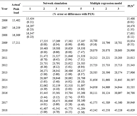
Numerical forecasting result and error comparison in term of Mean Absolute Percentage Error (MAPE) obtained from all network simulations and the multiple regression model are presented altogether with the actual peak load and with that made by PLN in Table 2 (Appendix).
4.1 LM-feedforward Network Structure
Simulations using the proposed network structure as described in the section 3.2 as well as using other structures with different number of neurons had been attempted. However, other network structure exhibited larger errors as the network output of 2006-2009 compared with its corresponding actual peak load.
All simulations applying the proposed network structure are described further in the following sections. Accordingly, comparison between network training and forecasting result either with actual peak load or with that made by PLN is shown graphically in each figure following to each simulation explanation.
Simulation-1
The actual historical data of 1995-2005 and actual peak load for the respective year is applied as the network input and training output target. Afterwards, network is simulated using data projection of 2006-2008 to obtain the corresponding peak load.
Fig. 1. Training and forecasting result of simulation-1. Fig. 2. Training and forecasting result of simulation-2.
Simulation-2
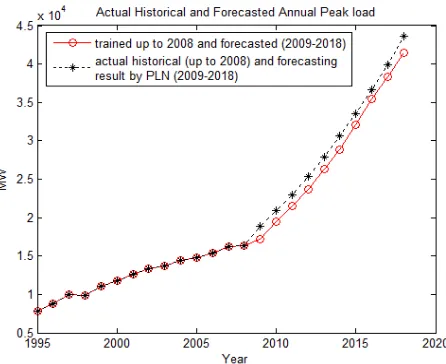
In this simulation, the same network structure as used in the simulation-1 is applied. Network input and training output target are actual historical data and actual peak load of 1995-2008, respectively. LTPF of 2009-2018 is obtained using the data projection of 2009-2018 as the network simulation input, including officially projected GRDP data during the forecasting period of 2009-2018.
Simulation-3
Network input is the same with that applied in simulation-2, which are actual historical data of 1995-2008. Meanwhile, slightly different target output is applied as the training output target are actual peak load of 1995-2005 and followed with the forecasted peak load of 2006-2008 obtained from simulation-1. LTPF of 2009-2018 is obtained using the same data projection as applied in simulation-2.
Simulation-4
Network input and training target output are are actual historical data of 1995-2008 and corresponding peak load as the training output target, respectively. LTPF of 2009-2018 with 5% additional to the officially projected GRDP is obtained considering higher GRDP growth.
Simulation-5
Network data set is the same with that applied in simulation-4. LTPF of 2009-2018 with 5% reduction to the officially projected GRDP during 2009-2018 is obtained from this simulation.
4.2 Multiple Regression Model
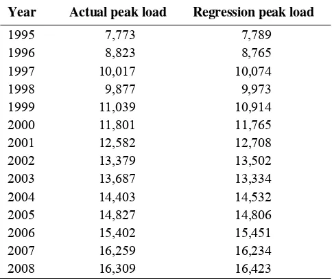
Comparison between actual historical peak load with that obtained by the Log-linear regression is given in Table 1.
load with respect to all data projection in the period of 2009-2018. The results, of which given in Table 2 (see Appendix), involved 3 economic growth scenario: (1)
officialy projected economic growth, (2) higher economic growth, and (3) lower economic growth.
Fig. 3. Training and forecasting result of simulation-3. Fig. 4. Training and forecasting result of simulation-4.
Fig. 5. Training and forecasting result of simulation-5.
Table 1. Actual and Double-log regression peak load
Year Actual peak load Regression peak load
1995 1996 1997 1998 1999 2000 2001 2002 2003 2004 2005 2006 2007 2008
7,773 8,823 10,017 9,877 11,039 11,801 12,582 13,379 13,687 14,403 14,827 15,402 16,259 16,309
4.3 Result comparison
Comparison in term of MAPE of the proposed network structure can be practically considered to be zero as exhibited in the training output during 1995-2008 whereas for Log-linear regression model is accounted for 0.75%. As presented in Table 2 (see Appendix), the network MAPE for simulation-1 (2006-2008) is 0.22%, of which far less than that projected by PLN, accounted for 3.16%. Likewise, the yearly errors exhibited by the network are tended to be steady whereas the PLN’s errors are excalated.
In 2009, forecating peak load of 17,269 MW, 18,788 MW, and 18,854 MW are exhibited by the proposed network (simulation-3), regression model, and PLN, respectively. The least forecasting error is obtained by the proposed network for 0.34%, followed by regression model and PLN, for 9.16% and 9.55%, respectively. In addition, results difference between the proposed network under simulation-2 and simulation-3 with that available from PLN are less than 7%, which is said to be acceptable for utility’s LTPF [14]. In term of network adaptability (see Table 2, Appendix), the simulation result is affected by applying changes in training output target as overall result exhibited by simulation-3 are slightly higher compared with that obtained by simulation-2.
Effect of GRDP variation on LTPF, economic growth can be observed accordingly from network simulation as well as multiple regression model. Overall forecasting peak load given by simulation-4 are higher in magnitude during 2009-2018, of which in the range of 157 MW to 366 MW, compared with that given by simulation-2. On the other hand, results obtained from simulation-5 are lower, in the range of 118 MW to 203 MW over the same forecasting period, compared with that achieved by simulation-2. Hence, the differences between network’s output and PLN’s projection are becoming larger than that in simulation-2. Meanwhile, the effect of GRDP variation in the Double-log regression model is not as significant as in the proposed network as the annual peak load forecasting differences between both higher and lower case to the base case are in the range of 7 MW to 16 MW.
5. CONCLUSION
ANN is characterized by (1) its architecture, (2) its training or learning algorithm, and (3) its activation function, for which the network performance would be mostly depend on, beside on the input variable selection and the network structure. Development of network structure involves decision making on type of network architecture and network size, in term of number of layers and neurons to be used. One reason for selecting a training algorithm is to speed up convergence and to avoid network from being trapped in the local minima.
In this paper, several simulations using the proposed LM-feedforward network have been conducted for LTPF problem of JaMaLi, Indonesia. The results exhibited by the network are much better in term of forecasting error than that given by the regression model and projection made by PLN. Regarding to the network
adaptability, applying different input and training output target has resulted variation of the network output in respective manner. Thus, the proposed network struture can be considered as promising alternative method for JaMaLi’s LTPF.
ACKNOWLEDGEMENT
Yusak Tanoto would like to express his gratitude to the Directorate General of Higher Education (DIKTI) under the Ministry of National Education of the Republic of Indonesia as the financier of this study.
REFERENCES
[1] Al-Saba, T. and El-Amin, I. 1999. Artificial neural networks as applied to long-term demand forecasting. Artificial Intelligence in Engineering 13: 189–197.
[2] Daneshi, H., Shahidehpour, M., and Choobbari, A.L. 2008. Long-term load forecasting in electricity market. In Proceedings of the IEEE International Conference on Electro/Information
Technology. Ames, Iowa, United States, 18-20
May. Pisctaway, NJ: Institute of Electrical and Electronics Engineer, Inc.
[3] Parlos, A.G. and Patton, A.D. 1993. Long-term electric load forecasting using a dynamic neural network architecture. In Proceedings of the Joint
International Power Conference. Athens, Greece,
5-8 September. Pisctaway, NJ: Institute of Electrical and Electronics Engineer, Inc.
[4] Hsu, C.C. and Chen, C.Y. 2003. Regional load forecasting in Taiwan–applications of artificial
neural networks. Energy Conversion and
Management, 44 (12): 1941-1949.
[5] Kuncoro, A.H., Zuhal, and Dalimi, R. 2007. Long-term peak load forecasting on the Java-Madura-Bali electricity system using artificial neural
network method. In Proceedings of the
International Conference on Advances in Nuclear Science and Engineering in Conjunction with
LKSTN. Bandung, 13-14 November. Jakarta:
Badan Tenaga Nuklir Nasional.
[6] Hagan, M.T. and Menhaj, M.B. 1994. Training Feedforward Networks with the Marquardt Algorithm. IEEE Transactions on Neural Networks 5(6): 989-993.
[7] PT. PLN (Persero). 2009. Press realease on 2008
achievement (in Bahasa Indonesia). Retrieved
September 4, 2009 from the World Wide Web:
http://www.pln.co.id/Portals/0/dokumen/PRESS% 20RELEASE%2017%20APRIL%202009%20(FIN
AL)..pdf.
[8] PT. PLN (Persero). 2009. PLN Statistics 2008. Jakarta: Corporate Secretary PT. PLN (Persero). [9] Center for Energy and Mineral Resources data
Information. 2009. Handbook of energy and
economic statistics of Indonesia 6th ed., 2008.
Jakarta: Ministry of Energy and Mineral Resources Republic of Indonesia.
Planning and Provision (RUPTL 2006-2015 - in
Bahasa Indonesia). Jakarta: Directorate of Planning
and Technology PT. PLN (Persero).
[11] PT. PLN (Persero). 2009. National Electricity Planning and Provision (RUPTL 2009-2018 - in
Bahasa Indonesia). Jakarta: Directorate of Planning
and Technology PT. PLN (Persero).
[12] Jadid, M.N. and Fairbairn, D.R. 1996. Predicting moment-curvature parameters from experimental data. Engineering Application Artifical Intelligence 9(3):303-319.
[13] Nguyen, D. And Widrow, B. 1990. Improving the learning speed of 2-layer neural networks by choosing initial values of the adaptive weights. In Proceedings of the International Joint Conference
on Neural Networks Volume 3. Washington DC,
United States, 15-19 January. Hillsdale: Lawrence Erlbaum Associates.
[14] Kermanshahi, B. and Iwamiya, H. 2002. Up to year 2020 load forecasting using neural nets. Electrical
Power and Energy System 24: 789-797.
APPENDIX
Table 2. Forecasting result and error comparison in percentage (MAPE)
Year
Actual* Peak
load
Network simulation Multiple regression model
PLN# 1 2 3 4 5 1 2 3
(% error or differences with PLN)
2006 15,402 15,434
(7.47) 20,870 20,878 20,863 20,900
2011 21,472
(7.31) 23,212 23,221 23,203 23,012
2012 23,731
(6.94) 25,723 25,733 25,713 25,343
2013 26,271
(6.37) 28,585 28,596 28,574 27,906
2014 28,867
(6.18) 31,656 31,668 31,645 30,597
2015 32,062
(4.88) 34,956 34,969 34,944 33,535
2016 35,445 35,561 35,704 35,268 38,111 38,124 38,097 36,708
2017
(5.56) 45,242 45,258 45,226 43,629