CFA 2018 Level 2 Quantitative methods

2017CFA

二级培训项目

Quantitative

Methods

周琪

工作职称：金程教育金融研究院CFA/FRM高级培训师

教育背景：中央财经大学国际经济学学士、澳大利亚维多利亚大学金融风 险管理学学士

工作背景：学术功底深厚、培训经验丰富，曾任课AFP、CFP多年，参与教

学研究及授课，现为金程教育CFA/FRM双证培训老师，担任CFA项目学术

研发负责人，对CFA教学产品的研发工作负责，曾亲自参与中国工商银行总

行、中国银行总行、杭州联合银行等CFA、FRM培训项目。累计课时达400 0小时，课程清晰易懂，深受学员欢迎。

服务客户：中国工商银行、中国银行、中国建设银行、杭州联合银行、杭 州银行、国泰君安证券、深圳综合开发研究院、中国CFP标准委员会、太平

Topic Weightings in CFA Level II

Session NO. Content Weightings

Study Session 1-2 Ethics & Professional Standards 10-15

Study Session 3 Quantitative Methods 5-10

Study Session 4 Economic Analysis 5-10

Study Session 5-6 Financial Statement Analysis 15-20

Study Session 7-8 Corporate Finance 5-15

Study Session 9-11 Equity Analysis 15-25

Study Session 12-13 Fixed Income Analysis 10-20

Study Session 14 Derivative Investments 5-15

Framework

Quantitative Methods

 SS3 Quantitative Methods for Valuation

• R9 Correlation and regression

• R10 Multiple regression and issues in regression analysis

• R11 Time-series analysis

• R12 Excerpt

from ’’Probabilistic

Approaches: Scenario

Analysis, Decision Trees, and

Reading

9

Framework

1. Scatter Plots

2. Covariance and Correlation

3. Interpretations of Correlation Coefficients 4. Significance Test of the Correlation

5. Limitations to Correlation Analysis 6. The Basics of Simple Linear Regression 7. Interpretation of regression coefficients 8. Standard Error of Estimate & Coefficient of

Determination (R2₎

9. Analysis of Variance (ANOVA)

10. Regression coefficient confidence interval 11. Hypothesis Testing about the Regression

Scatter Plots

Sample Covariance and Correlation



Covariance:



Covariance measures how one random variable moves with

another random variable. ----It captures the linear relationship.





Covariance ranges from negative infinity to positive infinity

Interpretations of Correlation Coefficients

 The correlation coefficient is a measure of linear association.

 It is a simple number with no unit of measurement attached, so the correlation coefficient is much easier to explain than the covariance.

Correlation coefficient Interpretation

r = +1 perfect positive correlation 0 < r < +1 positive linear correlation

r = 0 no linear correlation

−1 < r < 0 negative linear correlation

Significance Test of the Correlation

 Test whether the correlation between the population of two variables is equal to zero.

 H₀: ρ=0; H_A: ρ≠0 (Two-tailed test)

 Test statistic:

 Decision rule: reject H₀ if t>+t _critical, or t<- t _critical

 Conclusion: the correlation between the population of two variables is significantly different from zero.

2 2

r-0

r n-2

t=

, df = n-2

1-r

1-r

n-2

Example

 The covariance between X and Y is 16. The standard deviation of X is 4 and the standard deviation of Y is 8. The sample size is 20. Test the significance of the correlation coefficient at the 5% significance level.

 Solution :

 The sample correlation coefficient r = 16/(4×8) = 0.5. The t-statistic can be computed as:

The critical t-value for α=5%, two-tailed test with df=18 is 2.101.

Since the test statistic of 2.45 is larger than the critical value of

20 2

0.5 2.45

1 0.25

t    

Limitations to Correlation Analysis

 Outliers

 Outliers represent a few extreme values for sample observations.

Relative to the rest of the sample data, the value of an outlier may be extraordinarily large or small.

Limitations to Correlation Analysis

 Spurious correlation

 Spurious correlation refers to the appearance of a causal linear relationship

when, in fact, there is no relation. Certain data items may be highly

correlated purely by chance. That is to say, there is no economic explanation

for the relationship, which would be considered a spurious correlation.

 correlation between two variables that reflects chance relationships in a particular data set,

 correlation induced by a calculation that mixes each of two variables with a third (two variables that are uncorrelated may be correlated if

Limitations to Correlation Analysis

 Nonlinear relationships

 Correlation only measures the linear relationship between two variables,

so it dose not capture strong nonlinear relationships between variables.

 For example, two variables could have a nonlinear relationship such as

Y= (1-X) 3 _{and the correlation coefficient would be close to zero, which is}

The Basics of Simple Linear Regression



Linear regression allows you to use one variable to make predictions

about another

, test hypotheses about the relation between two

variables, and quantify the strength of the relationship between the

two variables.



Linear regression

assumes a linear relation between the dependent

and the independent variables.



The dependent variable is the variable whose variation is

explained by the independent variable. The dependent variable

is also refer to as

the explained variable, the endogenous

variable, or the predicted variable

.

The Basics of Simple Linear Regression

 The simple linear regression model

 Where

Y_i = ith observation of the dependent variable, Y

X_i = ith observation of the independent variable, X

b₀ = regression intercept term

b₁ = regression slope coefficient

ε_i= the residual for the ith observation (also referred to as the disturbance term or error term)

n

i

X

b

b

Interpretation of regression coefficients



Interpretation of regression coefficients



The

estimated intercept coefficient

( ) is interpreted as the

value of Y when X is equal to zero.



The

estimated slope coefficient

( ) defines the sensitivity of

Y to a change in X .The estimated slope coefficient ( ) equals

covariance divided by variance of X.



Example



An estimated slope coefficient of 2 would indicate that the

dependent variable will change two units for every 1 unit change

in the independent variable.

The assumptions of the linear regression

 The assumptions

 A linear relationship exists between X and Y

 X is not random, and the condition that X is uncorrelated with the error term can substitute the condition that X is not random.

 The expected value of the error term is zero (i.e., E(ε_i)=0 )

 The variance of the error term is constant (i.e., the error terms are homoskedastic)

 The error term is uncorrelated across observations (i.e., E(ε_iε_j)=0 for all i≠j)

Calculation of regression coefficients

 Ordinary least squares (OLS)

 OLS estimation is a process that estimates the population parameters B_i with corresponding values for b_i that minimize the squared residuals (i.e., error terms).

 the OLS sample coefficients are those that:

Example: calculate a regression coefficient

 Bouvier Co. is a Canadian company that sells forestry products to several Pacific Rim customers. Bouvier’s sales are very sensitive to exchange rates. The following table shows recent annual sales (in millions of Canadian dollars) and the average exchange rate for the year (expressed as the units of foreign currency needed to buy one Canadian dollar).

 Calculate the intercept and coefficient for an estimated linear

regression with the exchange rate as the independent variable and sales as the dependent variable.

Example: calculate a regression coefficient

 The following table provides several useful calculations:

Example: calculate a regression coefficient

 The sample mean of the exchange rate is:

 The sample mean of sales is:

 We want to estimate a regression equation of the form Y_i = b₀ + b₁X_i +ε_i. The estimates of the slope coefficient and the intercept are

ANOVA Table

 ANOVA Table

 Standard error of estimate:

 Coefficient of determination (R²)



 explained variation=1-unexplained variation

Standard Error of Estimate

 Standard Error of Estimate (SEE) measures the degree of variability of the

actual Y-values relative to the estimated Y-values from a regression equation.

 SEE will be low (relative to total variability) if the relationship is very strong

and high if the relationship is weak.

 The SEE gauges the “fit” of the regression line. The smaller the standard

error, the better the fit.

 The SEE is the standard deviation of the error terms in the regression.

MSE

n

SSE

SEE







Coefficient Determination (R

2

₎

 A measure of the “goodness of fit” of the regression. It is interpreted as a percentage of variation in the dependent variable explained by the independent variable. Its limits are 0≤R2≤_1.

 Example: R2 _{of 0.63 indicates that the variation of the independent}

variable explains 63% of the variation in the dependent variable.

 For simple linear regression, R² is equal to the squared correlation coefficient (i.e., R² = r² )

 The Different between the R2 _{and Correlation Coefficient}

 The correlation coefficient indicates the sign of the relationship between two variables, whereas the coefficient of determination does not.

Example

 An analyst ran a regression and got the following result:

 Fill in the blanks of the ANOVA Table.



ANOVA Table df SS MSS

Regression 1 8000 ?

Error ? 2000 ?

Total 51 ? -

Coefficient t-statistic p-value

Intercept -0.5 -0.91 0.18

Regression coefficient confidence interval

 Regression coefficient confidence interval

 If the confidence interval at the desired level of significance dose not

include zero, the null is rejected, and the coefficient is said to be statistically different from zero.

 is the standard error of the regression coefficient.

 As SEE rises, also increases, and the confidence interval widens because SEE measures the variability of the data about the regression line, and the more variable the data, the less confidence there is in the regression model to estimate a coefficient.

Hypothesis Testing about Regression Coefficient

 Significance test for a regression coefficient

 H₀: b₁=The hypothesized value(usually 0)

 Test Statistic:

 Decision rule: reject H₀ if +t _critical <t, or t<- t _critical

 Rejection of the null means that the slope coefficient is different from the hypothesized value of b₁.

Predicted Value of the Dependent Variable

 Predicted values are values of the dependent variable based on the

estimated regression coefficients and a prediction about the value of the independent variable.

 Point estimate

 Confidence interval estimate

Limitations of Regression Analysis

 Regression relations change over time

 This means that the estimation equation based on data from a specific time period may not be relevant for forecasts or predictions in another time period. This is referred to as parameter instability.

 The usefulness will be limited if others are also aware of and act on the relationship.

 Regression assumptions are violated

Reading

10

Framework

1. The Basics of Multiple Regression 2. Interpreting the Multiple Regression

Results

3. Hypothesis Testing about the Regression Coefficient

4. Regression Coefficient F-test 5. Coefficient of Determination (R2₎

6. Analysis of Variance (ANOVA) 7. Dummy variables

8. Multiple Regression Assumptions 9. Multiple Regression Assumption

Violations

The Basics of Multiple Regression

 Multiple regression is regression analysis with more than one independent variable

 The multiple linear regression model

X_ij = ith observation of the jth independent variable

N = number of observation

K = number of independent variables

 Predicted value of the dependent variable

Interpreting the Multiple Regression Results

 The intercept term is the value of the dependent variable when the

independent variables are all equal to zero.

 Each slope coefficient is the estimated change in the dependent variable for

a one unit change in that independent variable, holding the other

independent variables constant. That’s why the slope coefficients in a

Multiple Regression Assumptions

 The assumptions of the multiple linear regression

 A linear relationship exists between the dependent and independent variables

 The independent variables are not random ( OR X is not correlated with error terms). There is no exact linear relation between any two or more independent variables

 The expected value of the error term is zero (i.e., E(ε_i)=0 )

 The variance of the error term is constant (i.e., the error terms are homoskedastic)

 The error term is uncorrelated across observations (i.e., E(ε_iε_j)=0 for all i≠j)

Dummy variables

 To use qualitative variables as independent variables in a regression

 The qualitative variable can only take on two values, 0 and 1

 If we want to distinguish between n categories, we need n−1 dummy

Dummy variables

 Interpreting the coefficients

 Example: EPS_t = b₀ + b₁Q_1t + b₂Q_2t + b₃Q_3t + ϵ

 EPS_t = a quarterly observation of earnings per share

 The intercept term, represents the average value of EPS for the fourth quarter.

 The slope coefficient on each dummy variable estimates the difference in earnings per share (on average) between the respective quarter (i.e., quarter 1, 2, or 3) and the omitted quarter (the fourth quarter in this case).

Analysis of Variance (ANOVA)

 ANOVA Table

 Standard error of estimate

 Coefficient of determination (R²)

Adjusted R

2

 R2 _{and adjusted R}2

 R2 _{by itself may not be a reliable measure of the explanatory power of}

the multiple regression model. This is because R2 _{almost always}

increases as variables are added to the model, even if the marginal contribution of the new variables is not statistically significant.

Hypothesis Testing about Regression Coefficient

 Significance test for a regression coefficient

 H₀: b_j=0

 Test statistic: df = n-k-1

 p-value: the smallest significance level for which the null hypothesis can be rejected

 Reject H₀ if p-value<α

 Fail to reject H₀ if p-value>α

 Regression coefficient confidence interval



Regression Coefficient F-test

 An F-statistic assesses how well the set of independent variables, as a group, explains the variation in the dependent variable.

 An F-test is used to test whether at least one slope coefficient is significantly different from zero

 Define hypothesis:

Regression Coefficient F-test

 Decision rule

 Reject H₀ : if F (test-statistic) > F _c (critical value)

 Rejection of the null hypothesis at a stated level of significance indicates that at least one of the coefficients is significantly different than zero, which is interpreted to mean that at least one of the independent variables in the regression model makes a significant contribution on the explanation of the dependent variable.

 The F-test here is always a one-tailed test.

Unbiased and consistent estimator

 An unbiased estimator is one for which the expected value of the estimator

is equal to the parameter you are trying to estimate.

 If not, called as unreliable.

 A consistent estimator is one for which the accuracy of the parameter

Multiple Regression Assumption Violations

 Heteroskedasticity 异方差

 Heteroskedasticity refers to the situation that the variance of the error term is not constant (i.e., the error terms are not homoskedastic)

 Unconditional heteroskedasticity occurs when the heteroskedasticity is not related to the level of the independent variables, which means that it dose not systematically increase or decrease with the change in the

value of the independent variables. It usually causes no major problems with the regression.

 Conditional heteroskedasticity is heteroskedasticity, that is, variance of error term is related to the level of the independent variables.

Multiple Regression Assumption Violations

 Effect of Heteroskedasticity on Regression Analysis

 Not affect the consistency of regression parameter estimators

 Consistency: the larger the number of sample, the lower probability of error.

 The coefficient estimates (the ) are not affected.

 The standard errors are usually unreliable estimates.

 If the standard errors are too small, but the coefficient estimates themselves are not affected, the t-statistics will be too large and the null hypothesis of no statistical significance is rejected too often (一

类错误).

 The opposite will be true if the standard errors are too large. (二类错

误)

 The F-test is also unreliable.

ˆ

j

Multiple Regression Assumption Violations

 Detecting Heteroskedasticity

 Two methods to detect heteroskedasticity

 residual scatter plots (residual vs. independent variable)

 the Breusch-Pagen χ² test

H₀: No heteroskedasticity, one-tailed test

Chi-square test: BP = n×R_residual², df=k

注意：以误差项squred residuals和X做回归，R_residual²是此回

归的决定系数

Decision rule: BP test statistic should be small (χ²分布表）

Multiple Regression Assumption Violations

 Serial correlation (autocorrelation)序列相关，自相关

 Serial correlation (autocorrelation) refers to the situation that the error terms are correlated with one another

 Serial correlation is often found in time series data

 Positive serial correlation exists when a positive regression error in one time period increases the probability of observing regression error for the next time period.

 Negative serial correlation occurs when a positive error in one

Multiple Regression Assumption Violations

 Effect of Serial correlation on Regression Analysis

 Positive serial correlation → Type I error & F-test unreliable

 Not affect the consistency of estimated regression coefficients.

 Because of the tendency of the data to cluster together from observation to observation, positive serial correlation typically results in coefficient standard errors that are too small, which will cause the computed t-statistics to be larger.

 Positive serial correlation is much more common in economic and financial data, so we focus our attention on its effects.

Multiple Regression Assumption Violations

 Detecting Serial correlation

 Two methods to detect serial correlation

 residual scatter plots

 the Durbin-Watson test

H₀: No serial correlation

DW ≈ 2×(1−r) Decision rule

Multiple Regression Assumption Violations

 Detecting Serial correlation

 Two methods to detect serial correlation

 residual scatter plots

 the Durbin-Watson test

H₀: No positive serial correlation

DW ≈ 2×(1−r) Decision rule

Inconclusive _{Fail to reject null hypothesis of no} positive serial correlation

Reject H₀, conclude positive serial

Multiple Regression Assumption Violations

 Methods to Correct Serial correlation

 adjusting the coefficient standard errors (e.g., Hansen method): the Hansen method also corrects for conditional heteroskedaticity.

 The White-corrected standard errors are preferred if only heteroskedasticity is a problem.

Multiple Regression Assumption Violations



Multicollinearity



Multicollinearity refers to the situation that two or more

independent variables are highly correlated with each other



In practice, multicollinearity is often a matter of degree rather

than of absence or presence.



Two methods to detect multicollinearity



t-tests indicate that none of the individual coefficients is

significantly different than zero, while the F-test indicates

overall significance and the R² is high.



the absolute value of the sample correlation between any

Summary of assumption violations

Assumption

violation Impact Detection Solution

Conditional Heteroskeda

sticity

Type I /II error

① _{Residual scatter plots} ② _{Breusch-Pagen} χ²_-test

(BP = n×R²)

①_{robust standard errors}

(White-corrected standard errors)

② _{generalized least squares}

Positive serial correlation

Type I error

① _{Residual scatter plots} ② _{Durbin-Watson test}

(DW≈2×(1−r))

①_{robust standard errors}

(Hansen method)

②_{Improve the specification}

Model Misspecification

 There are three broad categories of model misspecification, or ways in which the regression model can be specified incorrectly, each with several

subcategories:

 1. The functional form can be misspecified.

 Important variables are omitted.

 Variables should be transformed.

 Data is improperly pooled.

 2. Time series misspecification. (Explanatory variables are correlated with the error term in time series models.)

 A lagged dependent variable is used as an independent variable with serially correlated errors.

 A function of the dependent variable is used as an independent variable ("forecasting the past").

Qualitative Dependent Variables

 Qualitative dependent variable is a dummy variable that takes on a value of either zero or one

 Probit and logit model: Application of these models results in estimates of the probability that the event occurs (e.g., probability of default).

 A probit model based on the normal distribution, while a logit model is based on the logistic distribution.

 Both models must be estimated using maximum likelihood methods

（极大似然估计）.

 These coefficients relate the independent variables to the likelihood of an event occurring, such as a merger, bankruptcy, or default.

 Discriminant models yields a linear function, similar to a regression

Credit Analysis



Z

–

score

Z = 1.2 A + 1.4 B + 3.3 C + 0.6 D + 1.0 E

Where:

A = WC / TA

B = RE / TA

C = EBIT / TA

D = MV of Equity / BV of Debt

E = Revenue / TA

Reading

11

Framework

1. Trend Models

2. Autoregressive Models (AR)

3. Random Walks

4. Autoregressive Conditional Heteroskedasticity (ARCH)

5. Regression with More Than One Time Series

Trend Models

 Linear trend model

 y_t=b₀+b₁t+ε_t

 Same as linear regression, except for that the independent variable is

time t (t=1, 2, 3, ……)

Trend Models

 Log-linear trend model

 y_t=e(b0+b1t)

 Ln(y_t )=b₀+b₁t+ε_t

 Model the natural log of the series using a linear trend

Trend Models

 Factors that Determine Which Model is Best

 A linear trend model may be appropriate if the data points appear to be

equally distributed above and below the regression line (inflation rate data).

 A log-linear model may be more appropriate if the data plots with a non-linear (curved) shape, then the residuals from a linear trend model will be persistently positive or negative for a period of time (stock

indices and stock prices).

 Limitations of Trend Model

 Usually the time series data exhibit serial correlation, which means that the model is not appropriate for the time series, causing inconsistent b₀ and b₁

Autoregressive Models (AR)

 An autoregressive model uses past values of dependent variables as independent variables

 AR(p) model

 AR (p): AR model of order p (p indicates the number of lagged values that the autoregressive model will include).

 For example, a model with two lags is referred to as a second-order autoregressive model or an AR (2) model.

0 1 1 2 2

...

t t t p t p t

Autoregressive Models (AR)

 Forecasting With an Autoregressive Model

 Chain rule of forecasting

 A one-period-ahead forecast for an AR (1) model is determined in the following manner:

 Likewise, a two-step-ahead forecast for an AR (1) model is calculated as:

1 0 1

t t

x

b

b x

  



 

2 0 1 1

t t

x

b

b x

  

Autoregressive Models (AR)



Forecasting With an Autoregressive Model, we should prove:



No autocorrelation



Covariance-stationary series

Autocorrelation

 Autocorrelation in an AR model

 Whenever we refer to autocorrelation without qualification, we mean autocorrelation of time series itself rather than autocorrelation of the error term .

 Detecting autocorrelation in an AR model

 Compute the autocorrelations of the residual

 t-tests to see whether the residual autocorrelations differ significantly from 0,

 If the residual autocorrelations differ significantly from 0, the model is not correctly specified, so we may need to modify it (e.g. seasonality)  Correction: add lagged values

Autocorrelation

 Seasonality – a special question

 Time series shows regular patterns of movement within the year

 The seasonal autocorrelation of the residual will differ significantly from

0

 We should uses a seasonal lag in an AR model

Example

 Suppose we decide to use an autoregressive model with a seasonal lag because of the seasonal autocorrelation in the previous problem. We are modeling quarterly data, so we estimate Equation:

 (ln Sales_t – ln Sales_t–1) = b₀ + b₁(ln Sales_t–1 – ln Sales_t–2) + b₂(ln Sales_t–4 – ln Sales_t–5) + ε_t.

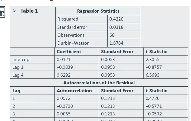
 Using the information in Table 1, determine if the model is correctly specified.

 Table 1

Table 1.Log Differenced Sales

Coefficient Standard Error t_-Statistic

Intercept 0.0121 0.0053 2.3055 Lag 1 –0.0839 0.0958 –0.8757 Lag 4 0.6292 0.0958 6.5693

Autocorrelations of the Residual

Lag Autocorrelation Standard Error t_-Statistic

Regression Statistics

Example

 Answer

 At the 0.05 significance level, with 68 observations and three parameters, this model has 65 degrees of freedom. The critical value of the t-statistic needed to reject the null hypothesis is thus about 2.0. The absolute value of the t-statistic for each

autocorrelation is below 0.60 (less than 2.0), so we cannot reject the null hypothesis that each autocorrelation is not significantly different from 0. We have determined that the model is correctly specified.

 If sales grew by 1 percent last quarter and by 2 percent four quarters ago, then the model predicts that sales growth this

quarter will be 0.0121 – 0.0839 ln(1.01) + 0.6292 ln(1.02) = e0.02372 –

Covariance-stationary

 Covariance-stationary series

 Statistical inference based on OLS estimates for a lagged time series model assumes that the time series is covariance stationary.

 Three conditions for covariance stationary

 Constant and finite expected value of the time series

 Constant and finite variance of the time series

 Constant and finite covariance with leading or lagged values

 Stationary in the past does not guarantee stationary in the future

Covariance-stationary

 Mean reversion

 A time series exhibits mean reversion if it has a tendency to move towards its mean

 For an AR(1) model, the mean reverting level is:

Covariance-stationary

 Instability of regression coefficients

 Financial and economic relationships are dynamic

 Models estimated with shorter time series are usually more stable than

those with longer time series

Random Walks

 Random walk

 Random walk without a drift

 Simple random walk: x_t =x_t-1+ε_t (b₀=0 and b₁=1)

 The best forecast of x_t is x_t-1

 Random walk with a drift

 x_t=b₀+x_t-1+ε_t (b₀≠0, b₁=1)

 The time series is expected to increase/decrease by a constant amount

 Features

 A random walk has an undefined mean reverting level

 A time series must have a finite mean reverting level to be covariance stationary

Unit root test

 The unit root test of nonstationarity

 The time series is said to have a unit root if the lag coefficient is equal to one

 A common t-test of the hypothesis that b₁=1 is invalid to test the unit root, however, it is not often the case.

 Dickey-Fuller test (DF test) to test the unit root

 Start with an AR(1) model x_t=b₀+b₁ x_t-1+ε_t

Subtract x_t-1 from both sides x_t-x_t-1 =b₀+(b₁ –1)x_t-1+ε_t

x_t-x_t-1 =b₀+gx_t-1+ε_t

Unit root correction



If a time series appears to have a unit root

 One method that is often successful is to first-difference the time series

(as discussed previously) and try to model the first-differenced series as

an autoregressive time series.



First differencing

 Define y_t as y_t = x_t - x_t-1 =ε_t

 This is an AR(1) model y_t = b₀ + b₁ y_t-1 +ε_t ,whereb₀=b₁=0

Autoregressive Conditional Heteroskedasticity

 Heteroskedasticity refers to the situation that the variance of the error term

is not constant.

 Test whether a time series is ARCH(1)



 If the coefficient a₁ is significantly different from 0, the time series is

ARCH(1), If a time-series model has ARCH(1) errors, then the variance of

the errors in period t + 1 can be predicted in period t.

 If ARCH exists,



多元回归中用BP test

2 2

0 1 1

t

a

a

t

u

t

Compare forecasting power with RMSE

 Comparing forecasting model performance

 In-sample forecasts are within the range of data (i.e., time period) used to estimate the model, which for a time series is known as the sample or test period.

 Out-of-sample forecasts are made outside. In other words, we compare how accurate a model is in forecasting the y variable value for a time period outside the period used to develop the model.

Regression with More Than One Time Series

 In linear regression, if any time series contains a unit root, OLS may be invalid

 Use DF tests for each of the time series to detect unit root, we will have 3 possible scenarios

 None of the time series has a unit root: we can use multiple regression

 At least one time series has a unit root while at least one time series does not: we cannot use multiple regression

 Each time series has a unit root: we need to establish whether the time series are cointegrated.

 If conintegrated, can estimate the long-term relation between the two series (but may not be the best model of the short-term

Regression with More Than One Time Series

 Use the Dickey-Fuller Engle-Granger test (DF-EG test) to test the

cointegration

 H₀: no cointegration H_a: cointegration

 If we cannot reject the null, we cannot use multiple regression

Steps in Time-Series Forecasting

画出散点图，判断序列是否有趋势

Does series have a trend?

No

a linear trend

指数趋势

an exponential trend

判断是否有季节性因素

Seasonality?

Steps in Time-Series Forecasting

Is series Covariance Stationary?

以差额法重新组建序列

Take First Differences

Reading

12

Framework

1. Simulation

Simulation

 Steps in Simulation

 Determine “probabilistic” variables

 Define probability distributions for these variables

 Historical data

 Cross sectional data

 Statistical distribution and parameters

 Check for correlation across variables

Simulation

 Advantage of using simulation in decision making

 Better input estimation

 A distribution for expected value rather than a point estimate

 Simulations with Constraints

 Book value constraints

 Regulatory capital restrictions

 Financial service firms

 Negative book value for equity

 Earnings and cash flow constraints

 Either internally or externally imposed

 Market value constraints

Simulation

 Issues in using simulation

 GIGO

 Real data may not fit distributions

 Non-stationary distributions

Comparing the Approaches

 Choose scenario analysis, decision trees, or simulations

 Selective versus full risk analysis

 Type of risk

 Discrete risk vs. Continuous risk

 Concurrent risk vs. Sequential risk

 Correlation across risk

 Correlated risks are difficult to model in decision trees Risk type and Probabilistic Approaches

Discrete/ Continuous

Correlated/ Independent

Sequential/

Concurrent Risk approach Discrete Correlated Sequential decision trees

It’s not the end but just beginning.

Life is short. If there was ever a moment to follow your passion and do

something that matters to you, that moment is now.