matter material after the index. Please use the Bookmarks
and Contents at a Glance links to access them.
v
Contents at a Glance
About the Author ...
xv
About the Technical Reviewer ...
xvii
Acknowledgments ...
xix
Foreword ...
xxi
Introduction ...
xxv
Chapter 1: Introduction to SQLTXPLAIN
■
...
1
Chapter 2: The Cost-Based Optimizer Environment
■
...
17
Chapter 3: How Object Statistics Can Make Your Execution Plan Wrong
■
...
39
Chapter 4: How Skewness Can Make Your Execution Times Variable
■
...
53
Chapter 5: Troubleshooting Query Transformations
■
...
71
Chapter 6: Forcing Execution Plans Through Profiles
■
...
93
Chapter 7: Adaptive Cursor Sharing
■
...
111
Chapter 8: Dynamic Sampling and Cardinality Feedback
■
...
129
Chapter 9: Using SQLTXPLAIN with Data Guard Physical Standby Databases
■
...
147
Chapter 10: Comparing Execution Plans
■
...
163
Chapter 11: Building Good Test Cases
■
...
177
Chapter 12: Using XPLORE to Investigate Unexpected Plan Changes
■
...
205
vi
Chapter 14: Running a Health Check
■
...
255
Chapter 15: The Final Word
■
...
281
Appendix A: Installing SQLTXPLAIN
■
...
285
Appendix B: The CBO Parameters (11.2.0.1)
■
...
295
Appendix C: Tool Configuration Parameters
■
...
307
xxv
Introduction
This book is intended as a practical guide to an invaluable tool called SQLTXPLAIN, commonly known simply as SQLT. You may never have heard of it, but if you have anything to do with Oracle tuning, SQLT is one of the most useful tools you’ll find. Best of all, it’s freely available from Oracle. All you need to do is learn how to use it.
How This Book Came to Be Written
I’ve been a DBA for over twenty years. In that time, I dealt with many, many tuning problems yet it was only when I began to work for Oracle that I learned about SQLT. As a part of the tuning team at Oracle Support I used SQLT every day to solve customers’ most complex tuning problems. I soon realized that my experience was not unique. Outside Oracle, few DBAs knew that SQLT existed. An even smaller number knew how to use it. Hence the need for this book.
Don’t Buy This Book
If you’re looking for a text on abstract tuning theory or on how to tune “raw” SQL. This book is about how to use SQLT to do Oracle SQL tuning. The approach used is entirely practical and uses numerous examples to show the SQLT tool in action.
Do Buy This Book
If you’re a developer or a DBA and are involved with Oracle SQL tuning problems. No matter how complex your system or how many layers of technology there are between you and your data, getting your query to run efficiently is where the rubber meets the road. Whether you’re a junior DBA, just starting your career, or an old hand who’s seen it all before, this book is designed to show you something completely practical that will be useful in your day-to-day work.
An understanding of SQLT will radically improve your ability to solve tuning problems and will also give you an effective checklist to use against new code and old.
1
Introduction to SQLTXPLAIN
Welcome to the world of fast Oracle SQL tuning with SQLTXPLAIN, or SQLT as it is typically called. Never heard of SQLT? You’re not alone. I’d never heard of it before I joined ORACLE, and I had been a DBA for more years than I care to mention. That’s why I’m writing this book. SQLT is a fantastic tool because it helps you diagnose tuning problems quickly. What do I mean by that? I mean that in half a day, maximum, you can go from a slow SQL to having an understanding of why SQL is malfunctioning, and finally, to knowing how to fix the SQL.
Will SQLT fix your SQL? No. Fixing the SQL takes longer. Some tables are so large that it can take days to gather statistics. It may take a long time to set up the test environment and roll the fix to production. The important point is that in half a day working with SQLT will give you an explanation. You’ll know why the SQL was slow, or you’ll be able to explain why it can’t go any faster.
You need to know about SQLT because it will make your life easier. But let me back up a little and tell you more about what SQLT is, how it came into existence, why you probably haven’t heard of it, and why you should use it for your Oracle SQL tuning.
What Is SQLT?
SQLT is a set of packages and scripts that produces HTML-formatted reports, some SQL scripts and some text files. The entire collection of information is packaged in a zip file and often sent to Oracle Support, but you can look at these files yourself. There are just over a dozen packages and procedures (called “methods”) in SQLT. These packages and procedures collect different information based on your circumstances. We’ll talk about the packages suitable for a number of situations later.
What’s the Story of SQLT?
They say that necessity is the mother of invention, and that was certainly the case with SQLT. Oracle support engineers handle a huge number of tuning problems on a daily basis; problem is, the old methods of linear analysis are just too slow. You need to see the big picture fast so you can zoom in on the detail and tell the customer what’s wrong. As a result, Carlos Sierra, a support engineer at the time (now a member of the Oracle Center of Expertise—a team of experts within Oracle) created SQLT. The routines evolved over many visits to customer sites to a point where they can gather all the information required quickly and effectively. He then provided easy-to-use procedures for reporting on those problems.
2
Why Haven’t You Heard of SQLT?
If it’s so useful, why haven’t you heard about SQLT? Oracle has tried to publicize SQLT to the DBA community, but still I get support calls and talk to DBAs who have never heard of SQLT—or if they have, they’ve never used it. This amazing tool is free to supported customers, so there’s no cost involved. DBAs need to look at problematic SQL often, and SQLT is hands down the fastest way to fix a problem. The learning curve may be high, but it’s nowhere near as high as the alternatives: interpreting raw 10046 trace files or 10053 trace files. Looking through tables of statistics to find the needle in the haystack, guessing about what might fix the problem and trying it out? No thanks. SQLT is like a cruise missile that travels across the world right to its target.
Perhaps DBAs are too busy to learn a tool, which is not even mentioned in the release notes for Oracle. It’s not in the documentation set, it’s not officially part of the product set either. It’s just a tool, written by a talented support engineer, and it happens to be better than any other tool out there. Let me repeat. It’s free.
It’s also possible that some DBAs are so busy focusing on the obscure minutiae of tuning that they forget the real world of fixing SQL. Why talk about a package that’s easy to use when you could be talking about esoteric hidden parameters for situations you’ll never come across? SQLT is a very practical tool.
Whatever the reason, if you haven’t used SQLT before, my mission in this book is to get you up and running as fast and with as little effort from you as possible. I promise you installing and using SQLT is easy. Just a few simple concepts, and you’ll be ready to go in 30 minutes.
How Did I Learn About SQLT?
Like the rest of the DBA world (I’ve been a DBA for many years), I hadn’t heard of SQLT until I joined Oracle. It was a revelation to me. Here was this tool that’s existed for years, which was exactly what I needed many times in the past, although I’d never used it. Of course I had read many books on tuning in years past: for example, Cary Millsaps’s classic Optimizing Oracle Performance, and of course Cost-Based Oracle Fundamentals by Jonathan Lewis.
The training course (which was two weeks in total) was so intense that it was described by at least two engineers as trying to drink water from a fire hydrant. Fear not! This book will make the job of learning to use SQLT much easier. Now that I’ve used SQLT extensively in day-to-day tuning problems, I can’t imagine managing without it. I want you to have the same ability. It won’t take long. Stick with me until the end of the book, understand the examples, and then try and relate them to your own situation. You’ll need a few basic concepts (which I’ll cover later), and then you’ll be ready to tackle your own tuning problems. Remember to use SQLT regularly even when you don’t have a problem; this way you can learn to move around the main HTML file quickly to find what you need. Run a SQLT report against SQL that isn’t a problem. You’ll learn a lot. Stick with me on this amazing journey.
Getting Started with SQLT
Getting started with SQLT couldn’t be easier. I’ve broken the process down into three easy steps.
1. Downloading SQLT
2. Installing SQLT
3. Running your first SQLT report
3
How Do You Get a Copy of SQLT?
How do you download SQLT? It’s simple and easy. I just did it to time myself. It took two minutes. Here are the steps to get the SQLT packages ready to go on your target machine:
1. Find a web browser and log in to My Oracle Support (http://support.oracle.com)
2. Go to the knowledge section and type “SQLT” in the search box. Note 215187.1 entitled “SQLT (SQLTXPLAIN) – Tool that helps to diagnose a SQL statement performing poorly [ID 215187.1]” should be at the top of the list.
3. Scroll to the bottom of the note and choose the version of SQLT suitable for your environment. There are currently versions suitable from 9i to 11 g.
4. Download the zip file (the version I downloaded was 2Mbytes).
5. Unzip the zip file.
You now have the SQLT programs available to you for installation onto any suitable database. You can download the zip file to a PC and then copy it to a server if needed.
How Do You Install SQLT?
So without further ado, let’s install SQLT so we can do some tuning:
1. Download the SQLT zip file appropriate for your environment (see steps above).
2. Unzip the zip file to a suitable location.
3. Navigate to your “install” directory under the unzipped area (in my case it is C:\Document and Settings\Stelios\Desktop\SQLT\sqlt\install, your locations will be different).
4. Connect as sys, e.g., sqlplus / as sysdba
5. Make sure your database is running
6. Run the sqcreate.sql script.
7. Select the default for the first option. (We’ll cover more details of the installation in Appendix A.)
8. Enter and confirm the password for SQLTXPLAIN (the owner of the SQLT packages).
9. Select the tablespace where the SQLTXPLAIN will keep its packages and data (in my case, USERS).
10. Select the temporary tablespace for the SQLTXPLAIN user (in my case, TEMP).
11. Then enter the username of the user in the database who will use SQLT packages to fix tuning problems. Typically this is the schema that runs the problematic SQL (in my case this is STELIOS).
12. Then enter “T”, “D” or “N.” This reflects your license level for the tuning and diagnostics packs. Most sites have both so you would enter “T”, (this is also the default). My test system is on my PC (an evaluation platform with no production capability) so I would also enter “T”. If you have the diagnostics pack, only enter “D”; and if you do not have these licenses, enter “N”.
4
Running Your First SQLT Report
Now that SQLT is installed, it is ready to be used. Remember that installing the package is done as sys and that running the reports is done as the target user. Please also bear in mind that although I have used many examples from standard schemas available from the Oracle installation files, your platform and exact version of Oracle may well be different, so please don’t expect your results to be exactly the same as mine. However, your results will be similar to mine, and the results you see in your environment should still make sense.
1. Now exit SQL and change your directory to ...\SQLT\run. In my case this is C:\Documents and Settings\Stelios\Desktop\SQLT\sqlt\run. From here log in to SQLPLUS as the target user.
2. Then enter the following SQL (this is going to be the statement we will tune):
SQL > select count(*) from dba_objects;
3. Then get the SQL_ID value from the following SQL
SQL > select sql_id from v$sqlarea where sql_text like 'select count(*) from dba_objects%';
In my case the SQL_ID was g4pkmrqrgxg3b.
4. Now we execute our first SQLT tool sqltxtract from the target schema (in this case STELIOS) with the following command:
SQL > @sqltxtract g4pkmrqrgxg3b
5. Enter the password for SQLTXPLAIN (which you entered during the installation). The last message you will see if all goes well is “SQLTXTRACT completed”.
6. Now create a zip directory under the run directory and copy the zip file created into the
zip directory. Unzip it.
7. Finally from your favorite browser navigate to and open the file named
sqlt_s <nnnnn> _main.html. The symbols “nnnnn” represent numbers created to make all SQLT reports unique on your machine. In my case the file is called sqlt_s89906_main.html
Congratulations! You have your first SQLT XTRACT report to look at.
When to Use SQLTXTRACT and When to Use SQLTXECUTE
5
Your First SQLT Report
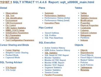
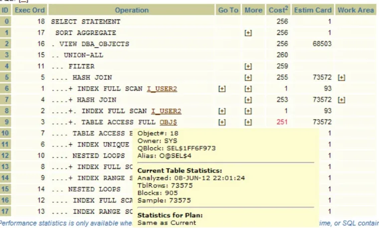
Before we get too carried away with all the details of using the SQLT main report, just look at Figure 1-1. It’s the beginning of a whole new SQLT tuning world. Are you excited? You should be. This header page is just the beginning. From here we will look at some basic navigation, just so you get an idea of what is available and how SQLT works, in terms of its navigation. Then we’ll look at what SQLT is actually reporting about the SQL.
Figure 1-1. The top part of the SQLT report shows the links to many areas
Some Simple Navigation
Before we get lost in the SQLT report let’s again look at the header page (Figure 1-1). The main sections cover all
Execution plan(s) (there will be more than one plan if the plan changed)
Take a minute and browse through the report.
Did you notice the hyperlinks on some of the data within the tables? SQLT collected all the information it could find and cross-referenced it all.
So for example, continuing as before from the main report at the top (Figure 1-1)
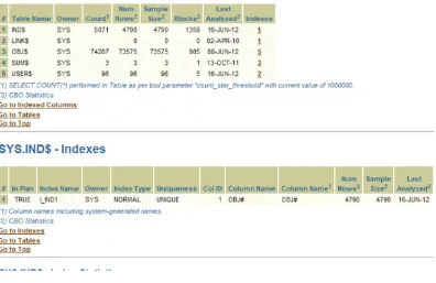
1. Click on Indexes, the last heading under Tables.
2. Under the Indexes column of the Indexes heading, the numbers are hyperlinked (see Figure 1-2). I clicked on 2 of the USERS$ record.
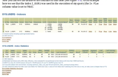
Now you can see the details of the columns in that table (see Figure 1-3). As an example here we see that the index I_USER2 was used in the execution of my query (the In Plan
column value is set to TRUE).
Figure 1-3. An Index’s detailed information about statistics
3. Now, in the Index Meta column (far right in Figure 1-3), click on the Meta hyperlink for the
Here we see the statement we would need to create this index. Do you have a script to do that? Well SQLT can get it better and faster. So now that you’ve seen a SQLT report, how do you approach a problem? You’ve opened the report, and you have one second to decide. Where do you go?
Well, that all depends.
How to Approach a SQLT Report
As with any methodology, different approaches are considered for different circumstances. Once you’ve decided there is something wrong with your SQL, you could use a SQLT report. Once you have the SQLT report, you are presented with a header page, which can take you to many different places (no one reads a SQLT report from start to finish in order). So where do you go from the main page?
If you’re absolutely convinced that the execution plan is wrong, you might go straight to “Execution Plans” and look at the history of the execution plans. We’ll deal with looking at those in detail later.
Suppose you think there is a general slowdown on the system. Then you might want to look at the “Observations” section of the report.
Maybe something happened to your statistics, so you’ll certainly need to look at the “Statistics” section of the report under “Tables.”
All of the sections I’ve mentioned above are sections you will probably refer to for every problem. The idea is to build up a picture of your SQL statement, understand the statistics related to the query, understand the cost-based optimizer (CBO) environment and try and get into its “head.” Why did it do what it did? Why does it not relate to what you think it ought to do? The SQLT report is the explanation from the optimizer telling you why it decided to do what it did. Barring the odd bug, the CBO usually has a good reason for doing what it did. Your job is to set up the environment so that the CBO agrees with your worldview and run the SQL faster!
Cardinality and Selectivity
My objective throughout this book, apart from making you a super SQL tuner, is to avoid as much jargon as possible and explain tuning concepts as simply as possible. After all we’re DBAs, not astrophysicists or rocket scientists.
So before explaining some of these terms it is important to understand why these concepts are key to the CBO operation and to your understanding of the SQL running on your system. Let’s first look at cardinality. It is defined as the number of rows expected to be returned for a particular column if a predicate selects it. If there are no statistics for the table, then the number is pretty much based on heuristics about the number of rows, the minimum and maximum values, and the number of nulls. If you collect statistics then these statistics help to inform the guess, but it’s still a guess. If you look at every single row of a table (collecting 100 percent statistics), it might still be a guess because the data might have changed, or the data may be skewed (we’ll cover skewness later). That dry definition doesn’t really relate to real life, so let’s look at an example. Click on the “Execution Plans” hyperlink at the top of the SQLT report to display an execution plan like the one shown in Figure 1-5.
In the “Execution Plan” section, you’ll see the “Estim Card” column. In my example, look at the TABLE ACCESS FULL OBJ$ step. Under the “Estim Card” column the value is 73,572. Remember cardinality is the number of rows returned from a step in an execution plan. The CBO (based on the table’s statistics) will have an estimate for the cardinality. The “Estim Card” column then shows what the CBO expected to get from the step in the query. The 73,572 shows that the CBO expected to get 73,572 records from this step, but in fact got 73,235. So how good was the CBO’s estimate for the cardinality (the number of rows returned for a step in an execution plan)? In our simple example we can do a very simple direct comparison by executing the query show below.
SQL> select count(*) from dba_objects; COUNT(*)
73235 SQL>
So cardinality is the actual number of rows that will be returned, but of course the optimizer can’t know the answers in advance. It has to guess. This guess can be good or bad, based on statistics and skewness. Of course, histograms can help here.
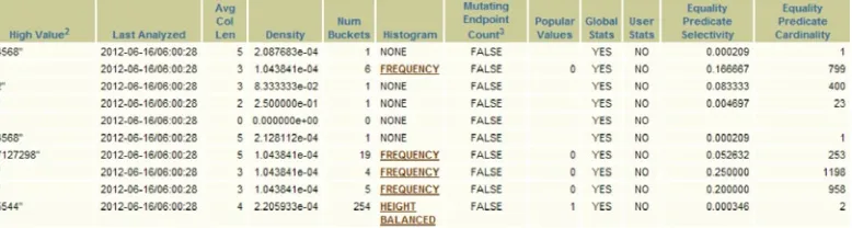
For an example of selectivity, let’s look at the page (see Figure 1-6) we get by selecting Columns from the Tables
options on the main page (refer to Figure 1-1).
Look at the “SYS.IND$ - Table Column” section. From the “Table Columns” page, if we click on the “34” under the “Column Stats” column, we will see the column statistics for the SYS.IND$ index. Figure 1-7 shows a subset of the page from the “High Value” column to the “Equality Predicate Cardinality” column. Look at the “Equality Predicate Selectivity” and “Equality Predicate Cardinality” columns (the last two columns). Look at the values in the first row for OBJ#.
Selectivity is 0.000209, and cardinality is 1.
This translates to “I expect to get 1 row back for this equality predicate, which is equivalent to a 0.000209 chance (1 is certainty 0 is impossible) or in percentage terms I’ll get 0.0209 percent of the entire table if I get the matching rows back.”
Notice that as the cardinality increases the selectivity also increases. The selectivity only varies between 0 and 1 (or if you prefer 0 percent and 100 percent) and cardinality should only vary between 0 and the total number of rows in the table (excluding nulls). I say should because these values are based on statistics. What would happen if you gathered statistics on a partition (say it had 10 million rows) and then you truncate that partition, but don’t tell the optimizer (i.e., you don’t gather new statistics, or clear the old ones). If you ask the CBO to develop an execution plan in this case it might expect to get 10 million rows from a predicate against that partition. It might “think” that a full table scan would be a good plan. It might try to do the wrong thing because it had poor information.
To summarize, cardinality is the count of expected rows, and selectivity is the same thing but on a 0–1 scale. So why is all this important to the CBO and to the development of good execution plans? The short answer is that the CBO is working hard for you to develop the quickest and simplest way to get your results. If the CBO has some idea about how many rows will be returned for steps in the execution plan, then it can try variations in the execution plan and choose the plan with the least work and the fastest results. This leads into the concept of “cost,” which we will cover in the next section.
What Is Cost?
Now that we have cardinality for an object we can work with other information derived from the system to calculate a cost for any operation. Other information from the system includes the following:
Speed of the disks
These metrics can be easily extracted from the system and are shown in the SQLT report also (under the “Environment” section). The amount of I/O and CPU resource used on the system for any particular step can now be calculated and thus used to derive a definite cost. This is the key concept for all tuning. The optimizer is always trying to reduce the cost for an operation. I won’t go into details about how these costs are calculated because the exact values are not important. All you need to know is this: higher is worse, and worse can be based on higher cardinality (possibly based on out-of-date statistics), and if your disk I/O speeds are wrong (perhaps optimistically low) then full table scans might be favored when indexes are available. Cost can also be directly translated into elapsed time (on a quiet system), but that probably isn’t what you need most of the time because you’re almost always trying to get an execution time to be reduced, i.e., lower cost. As we’ll see in the next section, you can get that information from SQLT. SQLT will also produce a 10053 trace file in some cases, so you can look at the details of how the cost calculations are made.
Reading the Execution Plan Section
We saw the execution plan section previously. It looks interesting, and it has a wobbly left edge and lots of hyperlinks. What does it all mean? This is a fairly simple execution plan, as it doesn’t go on for pages and pages (like SIEBEL or PeopleSoft execution plans).
There are a number of simple steps to reading an execution plan. I’m sure there’s more than one way of reading an execution plan, but this is the way I approach the problem. Bear in mind in these examples that if you are familiar with the pieces of SQL being examined, you may go directly to the section you think is wrong; but in general if you are seeing the execution plan for the first time, you will start by looking at a few key costs.
The first and most important cost is the overall cost of the entire query. This is always shown as “ID 0” and is always the first row in the execution plan. In our example shown in Figure 1-5, this is a cost of 256. So to get the cost for the entire query just look at the first row. This is also the last step to be executed (“Exec Ord” is 18). The execution order is not top to bottom, the Oracle engine will carry out the steps in the order shown by the value in the “Exec Ord” column. So if we followed the execution through, the Oracle engine would do the execution in this order:
1. INDEX FULL SCAN I_USER2
2. INDEX FULL SCAN I_USER2
3. TABLE ACCESS FULL OBJ$
4. HASH JOIN
5. HASH JOIN
6. INDEX UNIQUE SCAN I_IND1
7. TABLE ACCESS BY INDEX ROWID IND$
8. INDEX FULL SCAN I_USERS2
9. INDEX RANGE SCAN I_OBJ4
10. NESTED LOOP
11. FILTER
12. INDEX FULL SCAN I_LINK1
13. INDEX RANGE SCAN I_USERS2
14. NESTED LOOPS
15. UNION-ALL
16. VIEW DBA_OBJECTS
17. SORT AGGREGATE
18. SELECT STATEMENT
The “Operation” column is also marked with “+” and “–” to indicate sections of equal indentation. This is helpful in lining up operations to see which result sets an operation is working on. So, for example, it is important to realize that the HASH JOIN at step 5 is using results from steps 1, 4, 2, and 3. We’ll see more complex examples of these later. It is also important to realize that the costs shown are aggregate costs for each operation as well. So the cost shown on the first line is the cost for the entire operation, and we can also see that most of the cost of the entire operation came from step 3. (SQLT helpfully shows the highest cost operation in red). So let’s look at step 1 (as shown in Figure 1-5) in more detail. In our simple case this is
"INDEX FULL SCAN I_USER2"
Let’s translate the full line into English: “First get me a full index scan of index I_USERS2. I estimate 93 rows will be returned which, based on your current system statistics (Single block read time and multi-block read times and CPU speed), will be a cost of 1.”
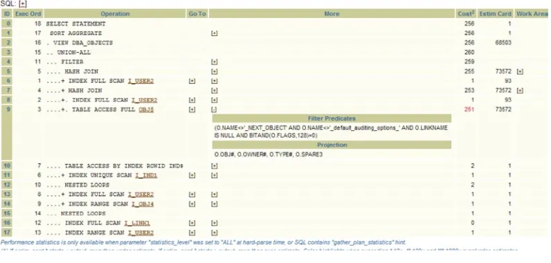
The second and third steps are another INDEX FULL SCAN and a TABLE ACCESS FULL of OBJ$. This third step has a cost of 251. The total cost of the entire SQL statement is 256 (top row). So if were looking to tune this statement we know that the benefit must come from this third step (it is a cost of 251 out of a total cost of 256). Now place your cursor over the word “TABLE” on step 3 (see Figure 1-8).
Notice how information is displayed about the object. Object#: 18
Owner: SYS
Qblock: SEL$1FF6F973
Alias: O@SEL$4 Current Table Statistics:
Analyzed: 08-JUN-12 22:01:24 TblRows: 73575
Blocks: 905 Sample 73575
Just by hovering your mouse over the object you get its owner, the query block name, when it was last analyzed, and how big the object is.
Now let’s look at the “Go To” column. Notice the “+” under that column? Click on the one for step 3, and you’ll get a result like the one in Figure 1-9.
15
So right from the execution plan you can go to the “Col Statistics” or the “Stats Versions” or many other things. You decide where you want to go next, based on what you’ve understood so far and on what you think is wrong with your execution plan. Now close that expanded area and click on the “+” under the “More” column for step 3 (see Figure 1-10)
Figure 1-10. Here we see an expansion under the “More” heading
Now we see the filter predicates and the projections. These can help you understand which line in the execution plan the optimizer is considering predicates for and which values are in play for filters.
Just above the first execution plan is a section called “Execution Plans.” This lists all the different execution plans the Oracle engine has seen for this SQL. Because execution plans can be stored in multiple places in the system, you could well have multiple entries in the “Execution Plans” section of the report. Its source will be noted (under the “Source” column). Here is a list of sources I’ve come across:
• GV$SQL_PLAN
• GV$SQLAREA_PLAN_HASH
• PLAN_TABLE
• DBA_SQLTUNE_PLANS
• DBA_HIST_SQL_PLAN
SQLT will look for plans in as many places as possible so that it can you give you a full range of options. When SQLT gathers this information, it will look at the cost associated with each of these plans and label them with “W” in red (worst) and “B” in green (best). In my simple test case, the “Best” and “Worst” are the same, as there is only one execution plan in play. However you’ll notice there are three records: one came from mining the memory
GV$SQL_PLAN, one came from PLAN_TABLE (i.e., an EXPLAIN PLAN) and one came from DBA_SQLTUNE_PLANS, (SQL Tuning Analyzer) whose source is DBA_SQLTUNE_PLANS.
Before we launch into even more detailed use of the “Execution Plans” section, we’ll need more complex examples.
Join Methods
This book is focused on very practical tuning with SQLT. I try to avoid unnecessary concepts and tuning minutiae. For this reason I will not cover every join method available or every DBA table that might have some interesting information about performance or every hint. These are well documented in multiple sources, not least of which is the Oracle Performance guide (which I recommend you read). However, we need to cover some basic concepts to ensure we get the maximum benefit from using SQLT. So, for example, here are some simple joins. As its name implies, a join is a way of “joining” two data sets together: one might contain a person’s name and age and another table might contain the person’s name and income level. In which case you could “join” these tables to get the names of people of a particular age and income level. As the name of the operation implies, there must be something to join the two data sets together: in our case, it’s the person’s name. So what are some simple joins? (i.e., ones we’ll see in out SQLT reports).
HASH JOINS (HJ) – The smaller table is hashed and placed into memory. The larger table is then scanned for rows that match the hash value in memory. If the larger and smaller tables are the wrong way around this is inefficient. If the tables are not large, this is inefficient. If the smaller table does not fit in memory, then this is more than inefficient: it’s really bad!
NESTED LOOP (NL)– Nested Loop joins are better if the tables are smaller. Notice how in the execution plan examples above there is a HASH JOIN and a NESTED LOOP. Why was each chosen for the task? The details of each join method and its associated cost can be determined from the 10053 trace file. It is a common practice to promote the indexes and NL by adjusting the optimizer parametersOptimizer_index_cost_adjandoptimizer_ index_cachingparameters. This is not generally a winning strategy. These parameters should be set to the defaults of 100 and 0. Work on getting the object and system statistics right first.
CARTESIAN JOINS – Usually bad. Every row of the first table is used as a key to access every row of the second table. If you have a very few number of rows in the joining tables this join is OK. In most production environments, if you see this occurring then something is wrong, usually statistics.
SORT MERGE JOINS (SMJ) – Generally joined in memory if memory allows. If the cardinality is high then you would expect to see SMJs and HJs.
Summary
In this chapter we covered the basics of using SQLTXTRACT. This is a simple method of SQLT that does not execute the SQL statement in question. It extracts the information required from all possible sources and presents this in a report.
The Cost-Based Optimizer
Environment
When I’m solving tricky tuning problems, I’m often reminded of the story of the alien who came to earth to try his hand at driving. He’d read all about it and knew the physics involved in the engine. It sounded like fun. He sat down in the driver’s seat and turned the ignition; the engine ticked over nicely, and the electrics were on. He put his seatbelt on and tentatively pressed the accelerator pedal. Nothing happened. Ah! Maybe the handbrake was on. He released the handbrake and pressed the accelerator again. Nothing happened. Later, standing back from the car and wondering why he couldn’t get it to go anywhere, he wondered why the roof was in contact with the road.
My rather strange analogy is trying to help point out that before you can tune something, you need to know what it should look like in broad terms. Is 200ms reasonable for a single block read time? Should system statistics be collected over a period of 1 minute? Should we be using hash joins for large table joins? There are 1,001 things that to the practiced eye look wrong, but to the optimizer it’s just the truth.
Just like the alien, the Cost Based Optimizer (CBO) is working out how to get the best performance from your system. It knows some basic rules and guestimates (heuristics) but doesn’t know about your particular system or data. You have to tell it about what you have. You have to tell the alien that the black round rubbery things need to be in contact with the road. If you ‘lie’ to the optimizer, then it could get the execution plan wrong, and by wrong I mean the plan will perform badly. There are rare cases where heuristics are used inappropriately or there are bugs in the code that lead the CBO to take shortcuts (Query transformations) that are inappropriate and give the wrong results. Apart from these, the optimizer generally delivers poor performance because it has poor information to start with. Give it good information, and you’ll generally get good performance.
So how do you tell if the “environment” is right for your system? In this chapter we’ll look at a number of aspects of this environment. We’ll start with (often neglected) system statistics and then look at the database parameters that affect the CBO. We’ll briefly touch on Siebel environments and the have a brief look at histograms (these are covered in more detail in the next chapter). Finally, we’ll look at both overestimates and underestimates (one of SQLT’s best features is highlighting these), and then we’ll dive into a real life example, where you can play detective and look at examples to hone your tuning skills (no peeking at the answer). Without further ado let’s start with system statistics.
System Statistics
workload is changing, for example from the daytime OLTP to a nighttime DW (Data Warehouse) environment, that different sets of system statistics should be loaded. In this section we’ll look at why these settings affect the optimizer, how and when they should be collected, and what to look for in a SQLT report.
Figure 2-1. The top section of the SQLT report
Let’s remind ourselves what the first part of the HTML report looks like (see Figure 2-1). Remember this is one huge HTML page with many sections.
From the main screen, in the Global section, select “CBO System Statistics”. This brings you to the section where you will see a heading “CBO System Statistics” (See Figure 2-2).
Now click on “Info System Statistics.” Figure 2-3 shows what you will see.
Figure 2-3. The “Info System Statistics” section
The “Info System Statistics” section shows many pieces of important information about your environment. This screenshot also shows the “Current System Statistics” and the top of the “Basis and Synthesized Values” section.
Notice, when the System Statistics collection was started. It was begun on 23rd of July 2007 (quite a while ago).
Has the workload changed much since then? Has any new piece of equipment been added? New SAN drives? Faster disks? All of these could affect the performance characteristics of the system. You could even have a system that needs a different set of system statistics for different times of the day.
The estimated SREADTIM (single block read time in ms.) and MREADTIM (multi-block read time in ms) are 12ms and 58ms, whereas the actual values (just below) are 3.4ms and 15ms. Are these good values? It can be hard to tell because modern SAN systems can deliver blistering I/O read rates. For traditional non-SAN systems you would expect multi-block read times to be higher than single block read times and the normally around 9ms and 22ms. In this case they are in a reasonable range. The Single block read time is less than the multi-block read time (you would expect that, right?).
Now look in Figure 2-5 at a screen shot from a different system.
Figure 2-4. From the “Basis and Synthesized Values” section just under “Info System Statistics” section
Notice anything unusual about the Actual SREADTIM and Actual MREADTIM?
Apart from the fact that the Actual SREADTIM is 6.809ms (a low value) and the Actual MREADTIM is 3.563ms (also a low value). The problem here is that the Actual MREADTIM is less than the SREADTIM. If you see values like these, you should be alert to the possibility that full table scans are going to be costed lower than operations that require single block reads.
What does it mean to the optimizer for MREADTIM to be less than SREADTIM? This is about equivalent to you telling the optimizer that it’s OK to drive the car upside down with the roof sliding on the road. It’s the wrong way round. If the optimizer takes the values in Figure 2-5 as the truth, it will favor steps that involve multi-block reads. For example, the optimizer will favor full table scans. That could be very bad for your run-time execution. If on the other hand you have a fast SAN system you may well have a low Actual MREADTIM.
The foregoing is just one example how a bad number can lead the optimizer astray. In this specific case you would be better off having no Actual values and relying on the optimizer’s guesses, which are shown as the estimated SREADTIM and MREADTIM values. Those guesses would be better than the actual values.
How do you correct a situation like I’ve just described? It’s much easier that you would think. The steps to fix this kind of problem are shown in the list below:
1. Choose a time period that is representative of your workload. For example, you could have a daytime workload called WORKLOAD.
2. Create a table to contain the statistics information. In the example below we have called the table SYSTEM_STATISTICS.
3. Collect the statistics by running the GATHER_SYSTEM_STATS procedure during the chosen time period.
4. Import those statistics using DBMS_STATS.IMPORT_SYSTEM_STATS.
Let’s look at the steps for collecting the system statistics for a 2-hour interval in more detail. In the first step we create a table to hold the values we will collect. In the second step we call the routine DBMS_STATS.GATHER_SYSTEM_STATS, with an INTERVAL parameter of 120 minutes. Bear in mind that the interval parameter should be chosen to reflect the period of your representative workload.
exec DBMS_STATS.CREATE_STAT_TABLE ('SYS','SYSTEM_STATISTICS'); BEGIN
DBMS_STATS.GATHER_SYSTEM_STATS ('interval',interval => 120, stattab => 'SYSTEM_STATISTICS', statid => 'WORKLOAD');
END; /
execute DBMS_STATS.IMPORT_SYSTEM_STATS(stattab => 'SYSTEM_STATISTICS', statid => 'WORKLOAD', statown => 'SYS');
Once you have done this you can view the values from the SQLT report or from a SELECT statement.
SYSSTATS_MAIN MREADTIM 55.901 SYSSTATS_MAIN CPUSPEED 972 SYSSTATS_MAIN MBRC
SYSSTATS_MAIN MAXTHR SYSSTATS_MAIN SLAVETHR
13 rows selected.
If you get adept at doing this you can even set up different statistics tables for different workloads and import them and delete the old statistics when not needed. To delete the existing statistics you would use
SQL> execute DBMS_STATS.DELETE_SYSTEM_STATS;
One word of caution, however, with setting and deleting system stats. This kind of operation will influence the behavior of the CBO for every SQL on the system. It follows therefore that any changes to these parameters should be made carefully and tested thoroughly on a suitable test environment.
Cost-Based Optimizer Parameters
Another input into the CBO’s decision-making process (for developing your execution plan) would be the CBO parameters. These parameters control various aspects of the cost based optimizer’s behavior. For example,
optimizer_dynamic_sampling controls the level of dynamic sampling to be done for SQL execution. Wouldn’t it be nice to have a quick look at every system and see the list of parameters that have been changed from the defaults? Well with SQLT that list is right there under “CBO Environment”.
Figure 2-6 is an example where almost nothing has been changed. It’s simple to tell this because there are only 2 rows in this section of the SQLT HTML report. The optimizer_mode has been changed from the default. If you see hundreds of entries here then you should look at the entries carefully and assess if any of the parameters that have been changed are causing you a problem. This example represents a DBA who likes to leave things alone.
Figure 2-6. The CBO environment section. Only 2 records indicates a system very close to the default settings
We also have 4 hidden parameters set (they are preceded by underscores). In this example each of the hidden parameters should be carefully researched to see if it can be explained. If you have kept careful records or commented on your changes you may know why _b_tree_bitmap_plans has been set to FALSE. Often, however, parameters like these can stay set in a system for years with no explanation.
The following are common explanations:
Somebody changed it a while ago, we don’t know why, and he/she has left now.
•
We don’t want to change it in case it breaks something.
•
This section is useful and can often give you a clue as to what has been changed in the past (perhaps you’re new to the current site). Take special note of hidden parameters. Oracle support will take a good look at these and decide if their reason for being still holds true. It is generally true that hidden parameters are not likely doing you any favors, especially if you don’t know what they’re for. Naturally, you can’t just remove them from a production system. You have to execute key SQL statements on a test system and then remove those parameters on that test system to see what happens to the overall optimizer cost.
Siebel Environment Considerations
Some environments are special just because Oracle engineering have decided that a special set of parameters are better for them. This is the case with Siebel Systems Customer Relationship Management (CRM) application. There are hidden parameters that Oracle engineering has determined get the best performance from your system. If your system is Siebel, then in the “Environment” section you will see something like that shown in Figure 2-8.
The “go to” place for Siebel tuning is the “Performance Tuning Guidelines for Siebel CRM Applications on Oracle Database” white paper. This can be found in Note 781927.1. There are many useful pieces of information in this document, but with regard to optimizer parameters, Page 9 lists the non-default parameters that should be set for good performance. For example, optimizer_index_caching should be set to 0.
Do not even attempt to tune your SQL on a Siebel system until these values are all correct. For example, on the above Siebel system if there was a performance problem, the first steps would be to fix all the parameters that are wrong according to Note 781927.1. You cannot hope to get stable performance from a Siebel CRM system unless this foundation is in place.
Hints
Hints were created to give the DBA and developer some control over what choices the optimizer is allowed to make. An example hint is USE_NL. In the example below I have created two minimal tables called test and test2, each with a single row. Not surprisingly if I let the optimizer choose a plan it will use a MERGE JOIN CARTESIAN as there are only single rows in each of these tables.
SQL> select 4 - filter("TEST"."COL1" = "TEST2"."COL1") Note
- dynamic sampling used for this statement (level=2) SQL> list
SQL> select /*+ USE_NL(test) */ * from test, test2 where test.col1=test2.col1;
- dynamic sampling used for this statement (level=2)
Notice how in the second execution plan a NESTED LOOP was used.
What we’re saying to the optimizer is: “we know you’re not as clever as we are, so ignore the rules and just do what we think at this point.”
Sometimes using hints is right, but sometimes it’s wrong. Occasionally hints are inherited from old code, and it is a brave developer who removes them in the hope that performance will improve. Hints are also a form of data input to the CBOs process of developing an execution plan. Hints are often needed because the other information fed to the optimizer is wrong. So, for example, if the object statistics are wrong you may need to give the optimizer a hint because its statistics are wrong.
Is this the correct way to use a hint? No. The problem with using a hint like this is that it may have been right when it was applied, but it could be wrong later, and in fact it probably is. If you want to tune code, first remove the hints, let the optimizer run free, while feeling the blades of data between its toes, free of encumbrances. Make sure it has good recent, statistics, and see what it comes up with.
You can always get the SQL Text that you are evaluating by clicking on the “SQL Text” link from the top section of the SQLT report. Here’s another example of a query. This time we’re using a USE_NL hint with two aliases
SQL> set autotrace traceonly explain; SQL> select cust_first_name, amount_sold 2 from customers C, sales S
3 where c.cust_id=s.cust_id and amount_sold>100; SQL> REM
Execution Plan
I’ve only shown part of the execution plan because we’re only interested in the operations (under the “Operation” column). Id 1 shows an operation of hash join. This is probably reasonable as there are over 900,000 rows in sales. The object with the most rows (in this case SALES) is read first and then CUSTOMERS (with only 55,500 rows). So if we decided to use a nested loop instead we would add a hint to the code like this:
The hint is enclosed inside “/*+” and “*/” as before. Anything inside these hint brackets will then be considered by the optimizer. But it is important to realize that the hint (in this case “USE_NL(C S)”) must be valid. Notice that now the operations have changed. Now the plan is to use nested loops instead of a hash join. The cost is much higher than the hash join plan at 145,000, but the optimizer has to obey the hint because it is valid. If it is not valid, no error is generated and the optimizer carries on as if there was no hint. Look at what happens.
SQL> select /*+ MY_HINT(C S) */ cust_first_name, amount_sold from
customers C, sales Swhere c.cust_id=s.cust_id and amount_sold>100;
Execution Plan
The optimizer saw my hint, didn’t recognize it as a valid hint, ignored it and did its own thing, which in this case was to go back to the hash join.
History of Changes
Look at the “Opt Env Hash Value” for the statement history in Figure 2-9. For the one SQL statement that we are analyzing with its list og “Begin Time” and “End Times” we see other changes taking place. For example, the plan hash value changed (for the same SQL statement) and so did the “Opt Env Hash Value”. Its value is 2904154100 until the 17th of February 2012. Then it changes to 3945002051 then back to 2904154100 and then back to 3945002051 (on the 18th of February). Something about the optimizer’s environment changed on those dates. Did the change improve the situation or make it worse? Notice that every time the optimizer hash value changes, the hash value of the plan changes also. Somebody or something is changing the optimizer’s environment and affecting the execution plan.
Column Statistics
One of the example SQLT reports (the first one we looked at) had the following line in the observation:
TABLE SYS.OBJ$ Table contains 4 column(s) referenced in predicates where the number of distinct values does not match the number of buckets.
If I follow the link to the column statistics (from the top section of the main HTML report, click on “Columns” then “Column Statistics”), I can see the results in Figure 2-10.
Figure 2-9. The optimizer Env Hash Value changed on the 22nd of February from 3945002051 to 2904154100. This
The second line of statistics is for the OWNER# table column. Look toward the right at the Num Distinct value. You’ll see that it is 30, representing that number of estimated distinct values. At the time the statistics were collected there probably were 30 or so distinct values. But notice the “Histogram” column! It shows a FREQUENCY type histogram with 25 buckets. In a FREQUENCY type histogram each possible value has a bucket in which is kept the number of values for that value. So for example if every value from 1 to 255 had only one value then each bucket would contain a “1”. If the first bucket (labeled “1” had 300 in it, this would mean that the value 1 had been found 300 times in the data. These numbers kept in the buckets are then used by the optimizer to calculate costs for retrieving data related to that value. So in our example above retrieving a “1” would be more costly than retrieving a “2” from the same table (because there are more values that are “1”s). If we had 10 buckets (each with their FREQUENCY value) and then we attempt to retrieve some data and find an “11”, then the optimizer has to guess that this new value was never collected and makes certain assumptions about the values likelihood (such as for higher and lower than the maximum values) the likelihood drops off dramatically as we go above the maximum value or below the minimum value. Values that have no buckets in the middle of the range are interpolated. So if you have less than 255 buckets, there is no good reason to have less than the actual number of buckets in a FREQUENCY histogram. That doesn’t make any sense. The result of this kind of anomaly is that the histogram information kept for the OWNER# column will have five distinct values missing. If the distinct values are popular, and if the query you are troubleshooting happens to use them in a predicate, the optimizer will have to guess their cardinality.
Imagine for example, the following situation:
1. Imagine a two bucket histogram with “STELIOS” and “STEVEN”. Now we add a third bucket “STEPHAN”, who happens to be the biggest owner of objects in OBJ$.
2. Let’s say the histogram values for STELIOS and STEVEN as follows: STELIOS – 100 objects
•
STEVEN – 110 objects
•
This means that for this particular table STELIOS has 100 records for objects he owns and
•
STEVEN has 110 objects that he owns. So when the histogram was created the buckets for STELIOS and STEVEN were filled with 100 and 110.
3. Further say that STEPHAN really owns 500 objects, so he has 500 records in the table. The optimizer doesn’t know that though, because STEPHAN was created at some point after statistics were collected.
The optimizer now guesses the cardinality of STEPHAN as 105, when in fact STEPHAN has 500 objects. Because STEPHAN falls between STELIOS and STEVEN (alphabetically speaking), the optimizer presumes the Num Distinct value for STEPHAN falls between the values for the other two users (105 is the average of the two adjacent, alphabetically speaking, buckets. The result is that the CBO’s guess for cardinality will be a long way out. We would see this in the execution plan (as an under estimate, if we ran a SQLT XECUTE), and we would drill into the OWNER# column and see that the column statistics were wrong. To fix the problem, we would gather statistics for SYS.OBJ$. In this case, of course, since the example we used was a SYS object there are special procedures for gathering statistics, but generally this kind of problem will occur on a user table and normal DBMS_STATS gathering procedures should be used.
Out-of-Range Values
The situation the CBO is left with when it has to guess the cardinality between two values is bad enough but is not as bad as the situation when the value in a predicate is out of range: either larger than the largest value seen by the statistics or smaller than the smallest value seen by the statistics. In these cases the optimizer assumes that the estimated value for the out of range value tails off towards zero. If the value is well above the highest value, the optimizer may estimate a very low cardinality, say 1. A cardinality of 1 might persuade the optimizer to try a Cartesian join, which would result in very poor performance if the actual cardinality was 10,000. The method of solving such a problem would be the same.
1. Get the execution plan with XECUTE.
2. Look at the execution plan in the Execution Plan section and look at the predicates under “more” as described earlier.
3. Look at the statistics for the columns in the predicates and see if there is something wrong. Examples of signs of trouble would be
a. A missing bucket (as described in the previous section)
b. No histograms but highly skewed data
Out-of-range values can be particularly troublesome when data is being inserted at the higher or lower ends of the current data set. In any case by studying the histograms that appear in SQLT you have a good chance of understanding your data and how it changes with time. This is invaluable information for designing a strategy to tune your SQL or collecting good statistics.
Over Estimates and Under Estimates
Now let’s look at a sample of a piece of SQL having so many joins that the number of operations is up to 96. See Figure 2-11, which shows a small portion of the resulting execution plan.
How do we handle an execution plan that has 96 steps, or more? Do we hand that plan over to development and tell them to tune it? With SQLT you don’t need to do this.
Let’s look at this page in more detail, by zooming in on the top right hand portion and look at the over and under estimates part of the screen (see Figure 2-12).
Figure 2-12. The top right hand portion of the section showing the execution plan’s over and under estimates
Figure 2-13. Over and under estimated values can be good clues
We know that Figure 2-12 is a SQLT XECUTE report, (we know this because we have over and under estimate values in the report). But what are these over and under estimates? The numbers in the “Last Over/Under Estimate” column, represent by how many factors the actual number of rows expected by the optimizer for that operation is wrong. The rows returned is also dependent on the rows returned from the previous operation. So, for example, if we followed the operation count step by step from “Exec Ord” (see Figure 2-11), we would have these steps:
1. INDEX RANGE SCAN actually returned 948 rows
2. INDEX RANGE SCAN actually returned 948 rows
3. The result of step 1 and 2 was fed into a NESTED LOOP which actually returned 948 rows
4. INDEX RANGE SCAN actually returned 948 rows
5. NESTED LOOP (of the previous step with result of step 3)
And so on. The best way to approach this kind of problem is to read the steps in the execution plan, understand them, look at the over and under estimates and from there determine where to focus your attention.
So for large statements like this, we work on each access predicate, each under and over estimate, working from the biggest estimation error to the smallest until we know the reason for each. In some cases, the cause will be stale statistics. In other cases, it will be skewed data. With SQLT, looking at a 200-line execution plan is no longer a thing to be feared. If you address each error as far as the optimizer is concerned (it expected 10 rows and got 1000) you can, step by step, fix the execution plan. You don’t need hints to twist the CBO into the shape you guess might be right. You just need to make sure it has good statistics for system performance, single and multiblock read times, CPU speed and object statistics. Once you have all the right statistics in place, the optimizer will generate a good plan. If the execution plan is sometimes right and sometimes wrong, then you could be dealing with skewed data, in which case you’ll need to consider the use of histograms. We discuss skewness as a special topic in much more detail in Chapter 4.
The Case of the Mysterious Change
Now that you’ve learned a little bit about SQLT and how to use it, we can look at an example without any prior knowledge of what the problem might be. Here is the scenario:
A developer comes to you and says his SQL was fine up until 3pm the previous day. It was doing
hash joins as he wanted and expected, so he went to lunch. When he came back the plan had
changed completely. All sorts of weird bit map indexes are being used. His data hasn’t changed,
and he hasn’t collected any new statistics. What happened? He ends by saying “Honest, I didn’t
change anything.”
Once you’ve confirmed that the data has not changed, and no-one has added any new indexes (or dropped any), you ask for a SQLT XECUTE report (as the SQL is fairly short running and this is a development system).
Once you have that you look at the execution plans. The plan in Figure 2-14 happens to be the one you view first.
Looking at the plan, you can confirm what the developer said about a “weird” execution plan with strange bit map indexes. In fact though, there is nothing strange about this plan. It’s just that the first step is:
... BITMAP INDEX FULL SCAN PRODUCTS_PROD_STATUS_BIX
This step was not in the developer’s original plan. Hence the reason the developer perceives it as strange. For the one SQL statement the developer was working with we suspect that there are at least 2 execution plans (there can be dozens of execution plans for the one SQL statement, and SQLT captures them all).
Further down in the list of execution plans, we see that there are indeed plans using hash joins and full table scans. See Figure 2-15, which shows a different execution plan for the same SQL that the developer is working with. In this execution plan, which returns the same rows as the previous execution plan, the overall cost is 908.
Figure 2-15. An execution plan showing a hash join
So far we know there was a plan involving a hash join and bitmap indexes and that earlier there were plans with full table scans. If we look at the times of the statistics collection we see that indeed the statistics were gathered before the execution of these queries. This is a good thing, as statistics should be collected before the execution of a query!
Note
■
As an aside, the ability of SQLT to present all relevant information quickly and easily is its greatest strength.
It takes the guesswork out of detective work. Without SQLT, you would probably have to dig out a query to show you
the time that the statistics were collected. With SQLT, the time of the collection of the statistics is right there in the report.
You can check it while still thinking about the question!
The objects section in Figure 2-16 will confirm the creation date of the index PRODUCTION_PROD_STATUS_BIX. As you can see, the index used in the BITMAP INDEX FULL SCAN was created long ago. So where are we now?
Let’s review the facts:
No new indexes have been added.
•
The plan has changed—it uses more indexes.
•
The statistics haven’t changed.
•
Now you need to consider what else can change an execution plan. Here are some possibilities:
System statistics. We check those, and they seem OK. Knowing what normal looks like
•
helps here.
Hints. We look to be sure. There are no hints in the SQL text.
•
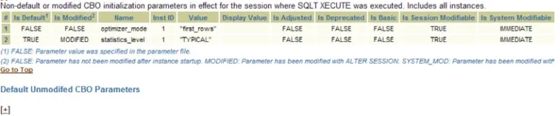
CBO parameters. We look and see the values in Figure
• 2-17.
Figure 2-17 shows statistics_level, _parallel_syspls_obey_force, and optimizer_index_cost_adj. This is in the section “Non-Default CBO Parameters”, so you know they are not normal values. As optimizer_index_cost_adj is a parameter for adjusting the cost used by the optimizer for indexes this may have something to do with our change in execution plan. Then notice that the “Observations” section (see Figure 2-18) highlights that there are non-standard parameters.
Figure 2-17. The CBO environment section
Figure 2-18. The “Observations” section of the HTML report shows non-default parameter observations, in this case 1 non-default parameter
If you look up optimizer_index_cost_adj, you will see that its default is 100 not 1. So now you have a working theory: The problem could lie with that parameter.
Now you can go to the users terminal, run his query, set the session value for optimizer_index_cost_adj to 100, re-run the query and see the different execution plan. We see the results below.
Execution Plan
---Plan hash value: 725901306
---Predicate Information (identified by operation id):
Now we have a cause and a fix, which can be applied to just the one session or to the entire system. The next step of course is to find out why optimizer_index_cost_adj was set, but that’s a different story, involving the junior DBA (or at least hopefully not you!) who set the parameter at what he thought was session level but turned out to be system level.
Summary
How Object Statistics Can Make Your
Execution Plan Wrong
In this chapter we’ll discuss what is considered a very important subject if you are tuning SQL. Gathering object statistics is crucial; this is why Oracle has spent so much time and effort making the statistics collection process as easy and painless as possible. They know that under most circumstances, DBAs who are under pressure to get their work done as quickly as possible, in the tiny maintenance windows they are allowed, will opt for the easiest and simplest way forward. If there is a check box that says “click me, all your statistics worries will be over,” they’ll click it and move on to the next problem.
The automated procedure has, of course, improved over the years, and the latest algorithms for automatically collecting statistics on objects (and on columns especially) are very sophisticated. However, this does not mean you can ignore them. You need to pay attention to what’s being collected and make sure it’s appropriate for your data structures and queries. In this chapter we’ll cover how partitions affect your plans and statistics capture. We’ll also look at how to deal with sampling errors and how to lock statistics and when this should be done. If this sounds boring, then that’s where SQLT steps in and makes the whole process simpler and quicker. Let’s start with object statistics.
What Are Statistics?
When SQL performs badly, poor-quality statistics are the most common cause. Poor-quality statistics cover a wide range of possible deficiencies:
Inadequate sample sizes.
•
Infrequently collected samples.
•
No samples on some objects.
•
Collecting histograms when not needed.
•
Not collecting histograms when needed.
•
Collecting statistics at the wrong time.
•
Collecting very small sample sizes on histograms.
•
Not using more advanced options like extended statistics to set up correlation between related
•
columns.
Relying on auto sample collections and not checking what has been collected.
It is crucial to realize that the mission statement of the cost-based optimizer (CBO) is to develop an execution plan that runs fast and to develop it quickly. Let’s break that down a little:
“Develop quickly.” The optimizer has very little time to parse or to get the statistics for the
•
object, or to try quite a few variations in join methods, not to mention to check for SQL optimizations and develop what it considers a good plan. It can’t spend a long time doing this, otherwise, working out the plan could take longer than doing the work.
“Runs fast.” Here, the key idea is that “wall clock time” is what’s important. The CBO is not
•
trying to minimize I/Os or CPU cycles, it’s just trying to reduce the elapsed time. If you have multiple CPUs, and the CBO can use them effectively, it will choose a parallel execution plan.
Chapter 1 discussed cardinality, which is the number of rows that satisfy a predicate. This means that the cost of any operation is made up of three operation classes:
Cost of single block reads
•
Cost of multi-block reads
•
Cost of the CPU used to do everything
•
When you see a cost of 1,000, what does that actually mean? An operation in the execution plan with a cost of 1,000 means that the time taken will be approximately the cost of doing 1,000 single-block reads. So in this case 1,000 x 12 ms, which gives 12 seconds (12 ms is a typical single- block read time).
So what steps does the CBO take to determine the best execution plan? In very broad terms the query is transformed (put in any shortcuts that are applicable), then plans are generated by looking at the size of the tables and deciding which table will be the inner and which will be the outer table in joins. Different join orders are tried and different access methods are tried. By “tried” I mean that the optimizer will go through a limited number of steps (its aim is to develop a plan quickly, remember) to calculate a cost for each of them and by a process of elimination get to the best plan. Sometimes the options the optimizer tries are not a complete list of plans, and this means it could miss the best plan; but this is extremely rare.
This is the estimation phase of the operation. If the operation being evaluated is a full table scan, this will be estimated based on the number of rows, the average length of the rows, the speed of the disk sub-system and so on.
Now that we know what the optimizer is doing to try and get you the right plan, we can look at what can go wrong when the object statistics are misleading.
Object Statistics
Object statistics are a vital input to the CBO, but even these can lead the optimizer astray when the statistics are out of date. The CBO also uses past execution history to determine if it needs better sampling (cardinality feedback) or makes use of bind peeking to determine which of many potential execution plans to use. Many people rely on setting everything on AUTO but this is not a panacea. If you don’t understand and monitor what the auto settings are doing for you, you may not spot errors when they happen.
Just to clarify, in the very simplest terms, why does the optimizer get it wrong when the statistics are out of date? After all once you’ve collected all that statistical information about your tables, why collect it again? Let’s do a thought experiment just like Einstein sitting in the trolley bus in Vienna.
Imagine you’ve been told there are few rows in a partition (<1,000 rows). You’re probably going to do a full table scan and not use the index, but if your statistics are out of date and you’ve had a massive data load (say 2.5 million rows) since the last time they ran and all of them match your predicate, then your plan is going to be sub-optimal. That’s tuning-speak for “regressed,” which is also tuning-speak for “too slow for your manager.” This underlines the importance of collecting statistics at the right time; after the data load, not before.
So far we’ve mentioned table statistics and how these statistics need to be of the right quality and of a timely nature. As data sets grew larger and larger over the years, so too did tables grow larger. Some individual tables became very large (Terabytes in size). This made handling these tables more difficult, purely because operations on these tables took longer. Oracle Corporation saw this trend early on and introduced table partitioning. These mini tables split a large table into smaller pieces partitioned by different keys. A common key is a date. So one partition of a table might cover 2012. This limited the size of these partitions and allowed operations to be carried out on individual partitions. This was a great innovation (that has a license cost associated with it) that simplified many day-to-day tasks for the DBA and allowed some great optimizer opportunities for SQL improvement. For example, if a partition is partitioned by date and you use a date in your predicate you might be able to use partition pruning, which only looks at the matching partitions. With this feature comes great opportunities for improvement in response times but also a greater possibility you’ll get it wrong. Just like tables, partitions need to have good statistics gathered for them to work effectively.
Partitions
Partitions are a great way to deal with large data sets, especially ones that are growing constantly. Use a range partition, or even better, an interval partition. These tools allow “old” data and “new” data to be separated and treated differently, perhaps archiving old data or compressing it. Whatever the reason, many institutions use