THESIS - MN142532
HEADING ANALYSIS OF WEATHERVANING
TURRET MOORED UNITS
FAHMY ARDHIANSYAH, ST NRP. 4115 203 002
SUPERVISOR Candidate
Aries Sulisetyono, Ph.D Wasis Dwi Aryawan, Ph.D
POST GRADUATE PROGRAME IN MARINE TECHNOLOGY CONCENTRATION IN SHIP HYDRODYNAMICS
FACULTY OF MARINE TECHNOLOGY
INSTITUT TEKNOLOGI SEPULUH NOPEMBER SURABAYA
iii
HEADING ANALYSIS OF WEATHERVANING TURRET
MOORED UNITS
Student Name : Fahmy Ardhiansyah, ST
ID Number : 4115 203 002
Supervisor : Aries Sulisetyono, Ph.D
Wasis Dwi Aryawan, Ph.D
ABSTRACT
This thesis report is present the heading study of weathervaning turret moored unit. With heading analysis over each of the sea states contained in time-series, mean heading of the floating structure can be obtained. Basically heading analysis will help the designer to perform analysis of structural strength, sloshing in tanks, green water prediction, loading/offloading operation, and fatigue life estimation. With heading analysis the designer will get a proper loading condition for their further analysis on weathervaning turret moored unit. Especially to optimized mooring system design based on heading analysis result which is will be performed in this thesis other than the heading analysis itself.
The result of heading analysis calculation indicated that the most affected external forces that causing vessel mean heading is dedicated by wind, it is seen the relative heading between wind and vessel heading is quite small (<10degree) with large occurrence probability (up to 45%). This probably due to the wind force coefficient is larger than current coefficient and also the wind age area is larger than hydrodynamic drag area.
Moreover the application of heading analysis considered in this study is for mooring system design. The result indicated that heading analysis is important to the designer to determine the pattern of anchor mooring. Nine (9) proposed mooring pattern has been investigated to check the mooring performance to withstand in rough water and fatigue life estimation as well in accordance to a well-known classification society.
v
PREFACE
Assalamu’alaikum Wr. Wb.
Indeed this work is due to Allah and for Allah… and Salawat on Prophet Muhammad and his family…
This thesis is submitted in order to complete the Master of Engineering (Magister Teknik) study in department of Naval Architecture and Shipbuilding Engineering at ITS Surabaya. This thesis have main concentration on Ship Hydrodynamic which is following by design of mooring system interest. This work was initiated from the author involvement during his job in ABADI MASELA FLNG project.
Hopefully this thesis will give encouragement to the reader which have intention in ship hydrodynamic and mooring system design. Moreover the MOSES software, which the academic license is given by Bentley Engineering to ITS, is one of the powerful hydrodynamic tools to solve quite complicated cases along the study. The syntax is also reported in this thesis report that will give another user to feel more enthusiast when he/she face a challenging hydrodynamic cases to solve.
Acknowledgements
The author would like to say thank you to everyone to their support, great comments, sharing of experience and knowledge that can improve encouragement to finish this research. At the moment author would say a very big thank you to this following figures:
1. My family; my wife: Mainas Ziyan Aghnia, my kids: Nusaibah and Ibrahim. You all
is my inspiration and my motivation, thanks for all full support and never ending encouragement to continue the study.
2. Ponorogo’s family and Gresik’s family; Yang Kung and Yang Ti also Aki and Uti.
It’s a pleasure to me to express my gratitude to all of you.
3. The supervisors: Bapak Aries Sulisetyono, Ph.D and Bapak Wasis Dwi Aryawan, Ph.D who give a lot of comments, discussion, and also great motivation.
4. All lecturer in Marine Technology Post Graduate Program: Achmad Zubaydi, Prof;
Djauhar Manfaat, Prof, IKAP Utama, Prof; Daniel M. Rosyid, Prof; Ketut Suastika, Dr; Herman Pratikno, Dr; Yeyes Mulyadi, Dr. Buana Ma’aruf, Prof.
5. Ocean Engineering Department peoples, especially: Rudi Waluyo, Dr; Murdjito, M.Eng; and also pak Murdjito and co., M. Kadafi, MT, Norman M. Sabana, ST. 6. Ship Design Laboratory in Department of Naval Architecture and Shipbuilding
Engineering peoples, especially:Achmad Baidowi, MT, Danu Utama, MT
7. Class of Boikot 2015 who spent an enjoying and relaxing moment along the study. This class will always suggest Boikot from a wrong doings to do a goodness for sure.
8. PTTI and PTGM colleague, especially: Daniel Ampulembang and Rudy Heryanto.
9. And everybody who cannot mention one by one in this report.
Finally, for finishing the study in ITS author could only wish may Allah reward you
with the best. ☺☺☺☺☺
Wassalamu’alaikum Wr. Wb.
Surabaya, January 2017
vii
2. LITERATURE STUDY AND THEORETICAL BACKGROUND ... 3
2.1 Literature Study ... 3
2.2 Theoretical Background ... 4
2.2.1 Wave Prediction and Climatology ... 4
2.2.2 Wind Loads ... 7
2.2.3 Current Loads ... 11
2.2.4 Wave Drift Forces and Moments ... 14
2.2.5 Sea Loads... 15
3.2.3 Wind and Current Load on Vessel ... 29
3.2.4 Wave Drift and Vessel Modelling ... 33
viii
3.5.5 Analysis Matrix and Load Cases ... 49
3.5.6 Design Criteria ... 52
4.3.1 Mooring Leg and Hull Clearance Analysis ... 80
4.3.2 Green Water and Chain Table Slamming Analysis ... 82
4.3.3 Mooring Line and Anchor Loads ... 83
4.3.4 Low Frequency Vessel Offset ... 99
4.3.5 Fatigue Life ... 100
5. CONCLUSION ... 105
ix
LIST OF FIGURES
Figure 2-1 Beaufort’s Wind Force Scale ... 4
Figure 2-2 Definitions Used here for Forces and Moments ... 9
Figure 2-3 Example of Wind Load Coefficients ... 10
Figure 3-1 Analysis Methodology ... 19
Figure 3-2 Relation between Wind Direction and Wind Speed ... 21
Figure 3-3 Annual Probability of Wind Direction ... 21
Figure 3-4 Relation between Current Direction and Current Speed ... 22
Figure 3-5 Annual Probability of Current Direction ... 22
Figure 3-6 Relation between Wind Wave Direction and Significant Wave Height ... 23
Figure 3-7 Annual Probability of Wind Wave Direction ... 23
Figure 3-8 Relation between Westerly Swell and Significant Wave Height ... 24
Figure 3-9 Annual Probability of Westerly Swell Direction ... 24
Figure 3-10 Relation between Peak Period and Significant Wave Height of Easterly Sea ... 25
Figure 3-11 Relation between Peak Period and Significant Wave Height of Westerly Sea ... 25
Figure 3-12 Relation between Peak Period and Significant Wave Height of Westerly Swell ... 26
Figure 3-13 Sign Convention Coordinate System ... 27
Figure 3-14 Wind Load Coefficients ... 29
Figure 3-15 Current Load Coefficients ... 29
Figure 3-16 Vessel Side Area ... 31
Figure 3-17 Vessel Front Area ... 31
Figure 3-18 Vessel Panel Model (totally 977 panels) ... 31
Figure 3-19 Heading Analysis Calculation Procedure ... 36
Figure 3-20 Equilibrium Calculation ... 38
Figure 3-21 Heading Analysis Algorithm ... 39
Figure 3-22 External Turret Mooring System Design ... 44
x
Figure 3-24 Schematic View of Mooring System ... 47
Figure 4-1 Quarter-seas RAO Compare to AQWA... 56
Figure 4-2 Added Mass Compare to WAMIT ... 57
Figure 4-3 Damping Compare to WAMIT ... 58
Figure 4-4 Vessel Motion Response Operator ... 61
Figure 4-5 Mean Drifting Forces ... 62
Figure 4-6 Heave Free Decay Test: Maximum for Each Cycles ... 65
Figure 4-7 Roll Free Decay Test: Maximum for Each Cycles ... 65
Figure 4-8 Pitch Free Decay Test: Maximum for Each Cycles ... 65
Figure 4-9 Weathervaning Analysis ... 70
Figure 4-10 Occurrence Probability of vessel’s Heading Angles ... 71
Figure 4-11 Relation between Wind Speed and Incident Wind Direction ... 72
Figure 4-12 Occurrence Probability of Wind Direction ... 72
Figure 4-13 Relation between Current Speed and Incident Current Direction ... 73
Figure 4-14 Occurrence Probability of Incident Current Direction ... 73
Figure 4-15 Relation between Significant Wave Height and Incident Wave Direction ... 74
Figure 4-16 Occurrence Probability of Incident Wave Direction ... 74
Figure 4-17 Relation between Significant Wave Height and incident Swell Direction ... 75
Figure 4-18 Occurrence Probability of Incident Swell Direction... 75
Figure 4-19 Wind and Current Area Comparison ... 76
Figure 4-20 Mooring Pattern Layout #1 ... 78
Figure 4-21 Elevation View of Vessel Bow and Anchor Leg: Calm Water. ... 81
Figure 4-22 200-yr Maximum Upstream Offset and Maximum Bow-Up Pitch. .. 81
Figure 4-23 3-Hour Simulation Relative Wave Elevation ... 82
Figure 4-24 Maximum Mooring Tension Load in Intact and Damage Cases ... 96
Figure 4-25 Environment Loadcase ... 97
Figure 4-26 Mooring Line Loads Summary ... 97
Figure 4-27 Vessel Low Frequency Offset: All Cases ... 99
Figure 4-28 Mooring Fatigue Design Curves ... 100
xi
LIST OF TABLES
Table 2-1 Turret Moored Units Typical and Behaviour ... 3
Table 3-1 Vessel Principal Particulars ... 28
Table 3-2 Wind Load Coefficients ... 30
Table 3-3 Current Load Coefficients ... 30
Table 3-4 Lateral Wind Screen for Topside ... 32
Table 3-5 Longitudinal Wind Screen for Topside ... 32
Table 3-6 Sample of MOSES Syntax ... 33
Table 3-7 A Sample Logging File to Estimate Heading Angles ... 40
Table 3-8 Geometry and Description ... 41
Table 3-9 Mooring Leg Properties ... 45
Table 3-10 Mooring Leg Lengths ... 45
Table 3-11 10-yr Return Period Environment Omni-Directional ... 48
Table 3-12 200-yr Return Period Environment Omni-Directional ... 48
Table 3-13 Mooring System Design Criteria ... 52
Table 4-1 Natural Period and Critical Damping ... 63
Table 4-2 Layout of Mooring Pattern ... 77
Table 4-3 Mooring Loads Summary Result ... 84
Table 4-4 Pile Anchor and Drag Anchor Design Load ... 87
1
1.
INTRODUCTION
1.1 Introduction
Design wave heading is to be in accordance with the operational conditions for the sea states contributing the most to the long term value of the dominant load effect (BV, 2010). The availability of berthing, connection, offloading and disconnection can be estimated on the basis of multi-vessel heading / mooring analysis for a significant amount of sea-states represented usually by time series of wind, current and wave (wind, sea & swell) over a large period of time (5 to 15 years: the larger the database, the better) (Jun, 2007)
From the heading analysis over each of the sea states contained in the time-series, the mean heading of the floating structure can be obtained. Then from the vessel heading, the relative heading of the vessel to the wind-sea, swell, wind and current could be derived, showing the trend of the floating structure behavior correlation with respect to the various metocean components. (Francois, 2004)
In the early 1960s, a new type of mooring system was developed for drillships. A rotating turret was inserted into the hull of The Offshore Company’s “Discoverer I” and mooring lines were extended out from the bottom of the turret and anchored to the seabed in a circular pattern. This SPM system allowed the drillship to continuously weathervane into the predominant seas without interrupting on-board drilling activities. At the same time SPM fluid-transfer systems (CALM buoy systems) were also being developed to allow easy offloading of liquids in shallow water offshore. The production “turret mooring system” evolved from these two concepts and was adapted to F(P)SO units that had to remain on location to provide a reliable means for storage and offloading for years without incurring significant downtime regardless of environmental conditions. Today, two types of turret systems are commonly used for F(P)SOs – the internal turret system where the turret is mounted within the F(P)SO hull, and an external turret system where the turret is mounted on an extended structure cantilevered off the vessel bow.(London, 2001)
2
From heading analysis algorithm as proposed by (T. Terashima, 2011) and (Morandini, 2007) the important point is an angle where the moment at the turret position is zero or near to zero, gives the balance heading angle of the vessel. Because the behavior of turret is free from moment that showing weathervaning effect. In this study the static approach by double check static equilibrium which is faster and easier way to get the heading angles result. A double check static equilibrium approach is believed can speed up computation without compromising the quality outcomes. It should be noted that dynamic equilibrium by time domain simulation in minimum 10,800s (3hrs) is still believed the most accurate, but time demanding consequences.
1.2 Problem Definitions
The problems are defined as follows:
1. The long-term response of weathervaneing turret moored floating unit in long-term seastate by heading analysis calculation.
2. The optimum mooring system design respect to heading analysis result.
1.3 Research Objective
The objective are defined as follows:
1. Assess heading analysis outcome as function of heading probability occurrences of weathervaning turret moored floating units.
2. Identify optimum mooring layout design respect to heading analysis result.
1.4 Research Question
The question are defined as follows:
‘How the importance of heading analysis in term of mooring system design is?’
1.5 Hypothesis
The hypothesis are defined as follows:
1. Numerous heading of floating unit will occurred relative to wave, wind, and current. 2. Heading analysis outcome will generated better hydrodynamic response condition
rather than a normal practice.
3
2.
LITERATURE STUDY AND THEORETICAL BACKGROUND
2.1 Literature Study
Heading analysis shall be necessary to be carried out for turret moored vessel unit. It was believed that such analysis would be a parameter for structural strength integrity and fatigue life estimation as well. Various hydrodynamic force and moment to be governed as per generated thousand number of sea state data respect to the scatter diagram. A fishtailing motions phenomenon would be occurred for single point moored units such a turret moored vessel due to time varying sea state. Failure of motions prediction will lead to lack of confidence for mooring design loads. Table 2.1 shown the behavior and typical of turret moored unit, it will be a prospect and constraint for this system depend on field condition (Howell, 2006).
Table 2-1 Turret Moored Units Typical and Behaviour
Turret-Moored
Vessel orientation 360 degree weathervaning
Environment Mild to extreme, directional to spread
Field layout Fairly adaptable, partial to distributed flow line
arrangements Riser number &
arrangement
Requires commitment, moderate expansion capability
Riser systems Location of turret (bow) requires robust riser design
Stationkeeping performance
Number of anchor legs, offset minimized
Vessel motions Weathervaning capability reduce motions
Vessel arrangement Turret provides “compact” load and fluid transfer system Offloading performance FPSO typically aligned with mean environment
4
Problems relating to weathervaning have been reported due to yaw instability in various Floating, Production, Storage and Offloading (FPSO) systems operating around the world thus disrupting the production/deck operations. Hydrodynamic analyses are economical means of analyzing the dynamics of a turret based system when subjected to different sea states. (Yadav, 2007)
As part of experiments a series of model tests in regular waves were conducted. Numerical computations for linear motion response of the FPSO were conducted using well established boundary element packages. It is found that the model deviated significantly from linear behavior in cases where there were involuntary heading changes. (Munipalli, 2007)
2.2 Theoretical Background
Theoretical background is refer to ref (Journée, 2001) as stated is Section 2.2.1 through Section 2.2.3 in this report. The theory are cover wave prediction and climatology, wind loads, current loads, and wave drift forces and moments.
2.2.1 Wave Prediction and Climatology
In 1805, the British Admiral Sir Francis Beaufort devised an observation scale for measuring winds at sea. His scale measures winds by observing their effects on sailing ships and waves. Beaufort’s scale was later adapted for use on land and is still used today by many weather stations. A definition of this Beaufort wind force scale is given in figure 2.1
5
Long Term Wave Prediction
Longer term wave climatology is used to predict the statistical chance that a given wave sensitive offshore operation - such as lifting a major top-side element into place - will be delayed by sea conditions which are too rough. The current section treats the necessary input data on wave climate.
In general, wave climatology often centers on answering one question: What is the chance that some chosen threshold wave condition will be exceeded during some interval – usually days, weeks or even a year? To determine this, one must collect - or obtain in some other way such as outlined in the previous section - and analyze the pairs of data (H1/3 and T) and possibly even including the wave direction, , as well) representing each ’storm’ period.
Wave Scatter Diagram
Sets of characteristic wave data values can be grouped and arranged in a table such as that given below based upon data from the northern North Sea. A ’storm’ here is an arbitrary time period - often of 3 or 6 hours - for which a single pair of values has been collected.
The number in each cell of this table indicates the chance (on the basis of 1000 observations in this case) that a significant wave height (in meters) is between the values in the left column and in the range of wave periods listed at the top and bottom of the table. Figure below shows a graph of this table.
Wave Climate Scatter Diagram for Northern North Sea
6
This scatter diagram includes a good distinction between sea and swell. As has already been explained early in this chapter, swell tends to be low and to have a relatively long period. The cluster of values for wave heights below 2 meters with periods greater than 10 seconds is typically swell in this case.
A second example of a wave scatter diagram is the table below for all wave directions in the winter season in areas 8, 9, 15 and 16 of the North Atlantic Ocean, as obtained from Global Wave Statistics.
These wave scatter diagrams can be used to determine the long term probability for storms exceeding certain sea states. Each cell in this table presents the probability of occurrence of its significant wave height and zero-crossing wave period range. This probability is equal to the number in this cell divided by the sum of the numbers of all cells in the table, for instance:
Pr{4 < 𝐻1/3 < 5and8 < 𝑇2 < 9} =999996 = 0.047 = 4.7%47072
For instance, the probability on a storm with a significant wave height between 4 and 6 meters with a zero-crossing period between 8 and 10 seconds is:
Pr{3 < 𝐻1/3< 5and8 < 𝑇2< 10} =47072 + 5643 + 74007 + 64809999996 = 0.242 = 24.2%
The probability for storms exceeding a certain significant wave height is found by adding the numbers of all cells with a significant wave height larger than this certain significant wave height and dividing this number by the sum of the numbers in all cells, for instance:
Pr{𝐻1/3 > 10} =6189 + 3449 + 1949 + 1116 + 1586999996 = 0.014 = 1.4%
7
quite different; think of an area in which there is a very pronounced hurricane season, for example. Statistically, the North Sea is roughest in the winter and smoothest in summer.
2.2.2 Wind Loads
Like all environmental phenomena, wind has a stochastic nature which greatly depends on time and location. It is usually characterized by fairly large fluctuations in velocity and direction. It is common meteorological practice to give the wind velocity in terms of the average over a certain interval of time, varying from 1 to 60 minutes or more. Local winds are generally defined in terms of the average velocity and average direction at a standard height of 10 meters above the still water level. A number of empirical and theoretical formulas are available in the literature to determine the wind velocity at other elevations. An adequate vertical distribution of the true wind speed z meters above sea level is represented by:
Vtw(z) = true wind speed at z meters height above the water surface Vtw(10) = true wind speed at 10 meters height above the water surface
Equation 2.1 is for sea conditions and results from the fact that the sea is surprisingly smooth from an aerodynamic point of view - about like a well mowed soccer field.
On land, equation 4.48 has a different exponent:
𝑉𝑡𝑤(𝑍)
𝑉𝑡𝑤(10)= (
𝑍
10)0.16 (on land) (2.2)
At sea, the variation in the mean wind velocity is small compared to the wave period. The fluctuations around the mean wind speed will impose dynamic forces on an offshore structure, but in general these aerodynamic forces may be neglected in comparison with the hydrodynamic forces, when considering the structures dynamic behavior. The wind will be considered as steady, both in magnitude and direction, resulting in constant forces and a constant moment on a fixed floating or a sailing body.
The wind plays two roles in the behavior of a floating body:
Its first is a direct role, where the wind exerts a force on the part of the structure exposed to the air. Wind forces are exerted due to the flow of air around the various parts. Only local winds are needed for the determination of these forces.
8
information about the wind and storm conditions in a much larger area. Wave and current generation is a topic for oceanographers; the effects of waves and currents on floating bodies will be dealt with separately in later chapters.
Only the direct influence of the winds will be discussed here.
Forces and moments will be caused by the speed of the wind relative to the (moving) body. The forces and moments which the wind exerts on a structure can therefore be computed by:
𝑋𝑤 =12 𝜌𝑎𝑖𝑟𝑉𝑟𝑤2 . 𝐶𝑋𝑤(𝛼𝑟𝑤). 𝐴𝑇
𝑌𝑤 = 12 𝜌𝑎𝑖𝑟𝑉𝑟𝑤2 . 𝐶𝑌𝑤(𝛼𝑟𝑤). 𝐴𝐿
𝑁𝑤 =12𝜌𝑎𝑖𝑟𝑉𝑟𝑤2 . 𝐶𝑁𝑤(𝛼𝑟𝑤). 𝐴𝐿. 𝐿 (2.3)
In which:
Xw = steady longitudinal wind force (N)
Yw = steady lateral wind force (N)
Nw = steady horizontal wind moment (Nm)
⍴air ⍴water/800 = density of air (kg/m3)
Vrw = relative wind velocity (m/s)
w = relative wind direction (-), from astern is
zero
AT = transverse projected wind area (m2)
AL = lateral projected wind area (m2)
L = length of the ship (m)
C*w(rw) = rw - dependent wind load coefficient (-) Note that it is a ”normal” convention to refer to the true wind direction as the direction from which the wind comes, while waves and currents are usually referred to in terms of where they are going. A North-West wind will cause South-East waves, therefore!
Wind Loads on Moored Ships
For moored ships, only the true wind speed and direction determine the longitudinal and lateral forces and the yaw moment on the ship, as given in figure 2.2. Because of the absence of a steady velocity of the structure, the relative wind is similar to the true wind:
9
Figure 2-2 Definitions Used here for Forces and Moments
The total force and moment experienced by an object exposed to the wind is partly of viscous origin (pressure drag) and partly due to potential effects (lift force). For blunt bodies, the wind force is regarded as independent of the Reynolds number and proportional to the square of the wind velocity.
(Remery and van Oortmerssen, 1973) collected the wind data on 11 various tanker hulls. Their wind force and moment coefficients were expanded in Fourier series as a function of the angle of incidence. From the harmonic analysis, it was found that a fifth order representation of the wind data is sufficiently accurate, at least for preliminary design purposes:
𝐶𝑋𝑤 = 𝑎0+ ∑ 𝑎𝑛sin(𝑛. 𝛼𝑟𝑤) 5
𝑛=1
𝐶𝑌𝑤 = ∑ 𝑏𝑛sin(𝑛. 𝛼𝑟𝑤) 5
𝑛=1
𝐶𝑁𝑤 = ∑5𝑛=1𝑐𝑛sin(𝑛. 𝛼𝑟𝑤) (2.5)
10
Figure 2.3 shows, as an example, the measured wind forces and moment together with their Fourier approximation, for one of the tankers.
Figure 2-3 Example of Wind Load Coefficients
Wind Loads on Other Moored Structures
11
2.2.3 Current Loads
There are several independent phenomena responsible for the occurrence of current: the ocean circulation system resulting in a steady current, the cyclical change in lunar and solar gravity causing tidal currents, wind and differences in sea water density. The steady wind velocity at the water surface is about 3 per cent of the wind velocity at 10 meters height. Tidal currents are of primary importance in areas of restricted water depth and can attain values up to 10 knots. However, such extreme velocities are rare; a 2-3 knots tidal current speed is common in restricted seas. The prediction of tidal currents is left for the oceanographers.
Although surface currents will be the governing ones for floating structures; the current distribution as a function of depth below the surface may also be of importance. For the design of a mooring system of a floating structure, the designer is especially interested in the probability that a particular extreme current velocity will be exceeded during a certain period of time. Observations obtained from current speed measurements are indispensable for this purpose. It may be useful to split up the total measured current in two or more components, for instance in a tidal and a non-tidal component, since the direction of the various components will be different, in general. The variation in velocity and direction of the current is very slow, and current may therefore be considered as a steady phenomenon. The forces and moment exerted by a current on a floating object is composed of the following parts:
A viscous part, due to friction between the structure and the fluid, and due to pressure drag. For blunt bodies the frictional force may be neglected, since it is small compared to the viscous pressure drag.
A potential part, with a component due to a circulation around the object, and one from the free water surface wave resistance. In most cases, the latter component is small in comparison with the first and will be ignored.
The forces and moments, as given in figure 2.2, exerted by the current on a floating structure can be calculated from:
𝑋𝑐 =12 𝜌. 𝑉𝑐2. 𝐶𝑋𝑐(𝛼𝑐). 𝐴𝑇𝑆
𝑌𝑐 = 12 𝜌𝑉𝑐2. 𝐶𝑌𝑐(𝛼𝑐). 𝐴𝐿𝑆
12 In which:
Xc = steady longitudinal current force (N)
Yc = steady lateral current force (N)
Nc = steady horizontal current moment (Nm)
⍴ = density of water (kg/m3)
Vc = relative current velocity (m/s)
c = relative current direction (-), from astern is
zero models of different sizes, tested at MARIN. The coefficients CXc, CY c and CNc were calculated from these results. A tanker hull is a rather slender body for a flow in the longitudinal direction and consequently the longitudinal force is mainly frictional. The total longitudinal force was very small for relatively low current speeds and could not be measured accurately. Moreover, extrapolation to full scale dimensions is difficult, since the longitudinal force is affected by scale effects.
For mooring problems the longitudinal force will hardly be of importance. An estimate of its magnitude can be made by calculating the flat plate frictional resistance, according to the ITTC skin friction line as given in equation:
13
L = length of the ship (m)
B = breadth of the ship (m)
T = draft of the ship (m)
Vc = current velocity (m/s)
c = current direction (-), from astern is zero
⍴ = density of water (ton/m3)
Rn = Reynolds number (-)
v = kinematic viscosity of water (m2s)
Extrapolation of the transverse force and yaw moment to prototype values is no problem. For flow in the transverse direction a tanker is a blunt body and, since the bilge radius is small, flow separation occurs in the model in the same way as in the prototype. Therefore, the transverse force coefficient and the yaw moment coefficient are independent of the Reynolds number.
The coefficients for the transverse force and the yaw moment were expanded by MARIN in a Fourier series, as was done for the wind load coefficients as described in a previous section:
𝐶𝑌𝑐 = ∑ 𝑏𝑛sin(𝑛. 𝛼𝑐) 5
𝑛=1
𝐶𝑁𝑐 = ∑5𝑛=1𝑐𝑛𝑠𝑖𝑛(𝑛. 𝛼𝑐) (2.10)
The average values of the coefficients bn and cn for the fifth order Fourier series, as published by (Remery and van Oortmerssen, 1973), are given in the table below.
14
dimensions change. For the condition to which these data apply, deep water and a prototype current speed in the order of 3 knots, the effect of the free surface is very small. For the case of a small clearance under the keel and a current direction of 90 degrees, damming up of the water at the weather side and a lowering of the water at the lee side of the ship occurs.
Current Loads on Other Moored Structures
Current loads on other types of floating structures are usually estimated in the same way as is used for wind loads.
2.2.4 Wave Drift Forces and Moments
15
Wave drifting forces in the horizontal directions, which are non-dimensionalzed can be calculated from:
When the size of the structure is comparable to the length of wave, the pressure on the structure may alter the wave field in the vicinity of the structure. In the calculation of wave forces, it is then necessary to account for the diffraction of the waves from the surface of the structure and the radiation of the wave from the structure if it moves (Chakrabarti, 1987).
First Order Potential Forces: Panel methods (also called boundary element methods, integral equation methods or sink-source methods) are the most common techniques used to analyze the linear steady state response of large-volume structures in regular waves (Faltinsen, 1990). They are based on potential theory. It is assumed that the oscillation amplitudes of the fluid and the body are small relative to cross-sectional dimension of the body. The methods can only predict damping due to radiation of surface waves and added mass. But they do not cover viscous effects. In linear analysis of response amplitude operator (RAO), forces and response are proportional to wave amplitude and response frequency are primarily at the wave frequency.
16
2.2.6 Floating Structure Dynamics
Dynamic response of an offshore structure includes the sea-keeping motion of the vessel in waves, the vibration of the structure, and the response of the moored systems. The response of an offshore structure may be categorized by frequency-content as below: Wave-frequency response: response with period in the range of 5 - 15 seconds. This is
the ordinary see-keeping motion of a vessel. It may be calculated using the firs-order motion theory.
Slowly-varying response: response with period in the range of 100 - 200 seconds. This is the slow drift motion of a vessel with its moorings. The slowly-varying response is of equal importance as the linear first-order motions in design of mooring and riser systems. Wind can also result in slowly-varying oscillations of marine structures with high natural periods. This is caused by wind gusts with significant energy at periods of the order of magnitude of a minute.
High-frequency response: response with period substantially below the wave period. For ocean-going ships, high frequency springing forces arise producing a high-frequency structural vibration that is termed whipping (Bhattacharyya, 1978). Owing to the high axial stiffness of the tethers, TLPs have natural periods of 2 to 4 seconds in heave, roll and pitch. Springing is a kind of resonance response to a harmonic oscillation (CMPT, 1998).
Impulsive response: Slamming occurs on the ship/platform bottoms when impulse loads with high-pressure peaks are applied as a result of impact between a body and water. Ringing of TLP tethers is a kind of transient response to an impulsive load. The high frequency response and impulsive response cannot be considered independently of the structural response. Hydroelasticity is an important subject.
2.2.7 Fatigue Analysis
Fundamentally, the fatigue analysis approaches in engineering applications can be subdivided into the following categories:
S-N based fatigue analysis approach
The local stress or strain approach where the calculation includes the local notch effects in addition to the general stress concentration
17
These approaches have been well implemented in the fatigue design and assessment. However, fatigue limit state design is still one of the most difficult topics in structural design, assessment or reassessment. For marine structures, additional complications arise because of the corrosive environment. The fundamental difficulties associated with fatigue problems are related to:
Lack of understanding of some of the underlying phenomena at both the microscopic and macroscopic levels
Lack of accurate information on the parameters affecting the fatigue life of a structure
19
There are three main step to perform heading analysis:
1. Collect and gather necessary data to enable proper heading analysis, ie environment data, vessel data, and another supporting data.
2. Build and generate numerical model of vessel by describing the capability to weathervane with respect to wind, current, and wave.
20
3.1 Environment Data
Metocean data are generally given in design data reports, in a statistical form that eliminates information of simultaneous occurrence of wave, wind, and current. Such information can be found on databases from hindcast or site measurements that normally form the source of design data. Such information is essential for any heading analysis and shall be provided for certain number of years, 2 years is believed being the absolute minimum.
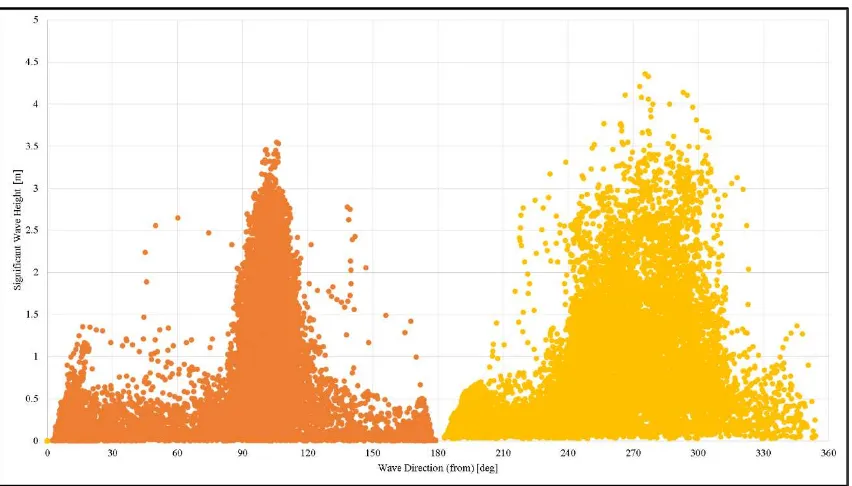
Environment data that will be used for this research are presented in Figure 3-2 through Figure 3-11, totally 28,209 cases. Direction of wind, current, wave/swell is defined zero when towards North and to increase Counter-Clockwise. The longterm analysis will be conducted to obtain several heading angles of the units and to optimize mooring system design purpose.
As can be seen in Figure 3-2 and Figure 3-3 the relation between wind direction and wind speed is presented. A lump easterly winds are prevailing in winter and westerly winds are prevailing in summer. A strong wind more than 15 m/s (29 knots) are occurred mainly for westerly winds.
Current data are available in Figure 3-4 and Figure 3-5 show the relation between wind direction and wind speed, also the annual probability of them. Where easterly current and northerly current mainly to prevail.
Wind wave data are shown in Figure 3-6 and Figure 3-7, the relation between wave direction and significant wave height. Wave data are divided onto easterly waves and westerly wave. In the referring Figure, total annual probability of easterly waves is 100% and respectively for westerly waves. The figure showing two waves system are coexisting. Maximum value of significant wave height of westerly waves is larger than easterly waves because of stronger westerly waves winds.
Swell occurrence as shown in Figure 3-8 and Figure 3-9 is almost limited to 240deg South West. Swell height is predicted up to 3.18 meter, which implies that large roll motions will be attributed to large swell.
21
Figure 3-2 Relation between Wind Direction and Wind Speed
Figure 3-3 Annual Probability of Wind Direction
0% 1% 2% 3% 4% 5% 6% 7% 8%
0 15 30 45 60 75 90 105 120 135 150 165 180 195 210 225 240 255 270 285 300 315 330 345 360
Pr
obab
il
ity
22
Figure 3-4 Relation between Current Direction and Current Speed
Figure 3-5 Annual Probability of Current Direction
0.0% 0.5% 1.0% 1.5% 2.0% 2.5% 3.0% 3.5% 4.0% 4.5%
0 15 30 45 60 75 90 105 120 135 150 165 180 195 210 225 240 255 270 285 300 315 330 345 360
Pr
obab
il
ity
23
Figure 3-6 Relation between Wind Wave Direction and Significant Wave Height
Figure 3-7 Annual Probability of Wind Wave Direction
0% 5% 10% 15% 20% 25%
0 15 30 45 60 75 90 105 120 135 150 165 180 195 210 225 240 255 270 285 300 315 330 345 360
O
cc
u
ren
ce
Prob
ab
il
ity
24
Figure 3-8 Relation between Westerly Swell and Significant Wave Height
Figure 3-9 Annual Probability of Westerly Swell Direction
0% 5% 10% 15% 20% 25% 30% 35% 40% 45% 50%
0 15 30 45 60 75 90 105 120 135 150 165 180 195 210 225 240 255 270 285 300 315 330 345 360
Oc
cu
rence
Pr
obab
il
ity
25
Figure 3-10 Relation between Peak Period and Significant Wave Height of Easterly Sea
26
27
3.2 Numerical Model
In order to perform heading analysis, the numerical model of the floating unit were generated which basically is the mooring analysis model. A 3D-diffraction software MOSES is used in this analysis. Details of MOSES software capabilities and analysis methodology are given in MOSES Manual (Ultramarine, 2012). The numerical model will be determine the characteristic of the unit with respect to wind, wave, and current that to be described as accurately possible with special care regarding the definition of reference points for numerous events.
3.2.1 Analysis Coordinate System
Figure 3-13 Sign Convention Coordinate System
First of all, prior to generate the numerical computation it should be determined the coordinate system. The sign conventions utilized for the analysis of motions and loads in earth-fixed and vessel-fixed local coordinate systems are defined below and are also shown in Figure 3-13.
Earth-fixed coordinate system (EFCS):
o The global X axis is coincident with the geographical North. o The global Y axis is coincident with the geographical West.
28 Vessel-fixed coordinate system (VFCS):
o The x-axis is along the vessel centerline, with x=0 at vessel origin and positive to stern.
o The y-axis is positive towards the starboard side of the vessel, with y=0 at the vessel center line.
o The z-axis is vertically upwards, with z=0 at the vessel keel.
Note that plan view angles increase in a counter-clockwise (CCW) fashion. Unless otherwise noted, both in the analysis and presentation of results, wind, wave and current angles refer to the directions towards which these environments propagate (i.e. heading) in the present EFCS system. Additionally, a relative wave heading of 0deg. corresponds to waves approaching the vessel stern-on, while a relative wave heading of 90deg. corresponds to waves approaching the vessel on the starboard beam.
3.2.2 Vessel Information
A box-shaped vessel with principal particular of turret moored unit in ballast draft operating condition are presented in Table 3-1.
29
3.2.3 Wind and Current Load on Vessel
Wind and current load basic theory are already stated in Section 2.2.2 and Section 2.2.3 in previous chapter. The wind and current coefficient that will be implemented in this
analysis shall be better from wind tunnel test experiment. Currently author can’t do such
experiment and also can’t get sufficient data regarding this issue, so in this research wind and current forces coefficient are assumed based on OCIMF recommendation. Further reading as more information can be seen in Prediction of Wind and Current Loads on VLCCs (OCIMF, 1994).
Figure 3-14 Wind Load Coefficients
30
Current and wind coefficients will be used for this analysis can be seen in Figure 3-14 and Figure 3-15. The angels are relative heading between vessel and wind/current heading defined in VFCS, i.e 0deg is stern-on and 90deg is beam-on from starboard. Corresponding value can be found in Table 3-2 and Table 3-3.
Table 3-2 Wind Load Coefficients
31
body present by green line. Respectively red line represent living quarter, topside module, flare tower, and turret structure.
Figure 3-16 Vessel Side Area
Figure 3-17 Vessel Front Area
32
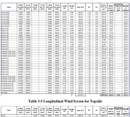
Table 3-4 Lateral Wind Screen for Topside
Table 3-5 Longitudinal Wind Screen for Topside
A total topside windage area in lateral and frontal is presented in Table 3-4 and Table 3-5. As can be seen the windage area is about 16,000 m2 and 1,000 m2 for lateral and longitudinal respectively. Furthermore the freeboard hull lateral and longitudinal windage area is about 9,900 m2 and 1,700 m2 respectively. Summing the lateral and longitudinal windage area is 26,640 m2 and 2,802 m2.
Turret [1/6] -50765 -10964 45061 53941 39.80 8.88 353.43 1.00 1.00 353.43 -30.86 49.50
Turret [2/6] -50765 -15229 53941 60706 35.54 6.77 240.40 1.00 1.00 240.40 -33.00 57.32
Turret [3/6] -50765 -18701 60706 69328 32.06 8.62 276.46 1.00 1.00 276.46 -34.73 65.02
Turret [4/6] -50765 -22490 69328 74946 28.28 5.62 158.85 1.00 1.00 158.85 -36.63 72.14
Turret [5/6] -49409 -24335 74946 81694 25.07 6.75 169.20 1.00 1.00 169.20 -36.87 78.32
Turret [6/6] -48464 -26558 81694 88007 21.91 6.31 138.29 1.00 1.00 138.29 -37.51 84.85
Flare Tower 3380 21285 38500 131951 17.91 93.45 1673.24 1.30 1.50 3262.82 12.33 85.23
Block A [1] 31885 57787 38500 83401 25.90 44.90 1163.03 1.00 1.00 1163.03 44.84 60.95
Block A [2] 62355 90866 38500 73184 28.51 34.68 988.88 1.00 1.00 988.88 76.61 55.84
Block A [3] 71269 84225 73184 95634 12.96 22.45 290.86 1.00 1.00 290.86 77.75 84.41
Block A [4] 90866 108635 38500 69674 17.77 31.17 553.93 1.00 1.00 553.93 99.75 54.09
Block A [5] 108635 139209 38500 71930 30.57 33.43 1022.09 1.00 1.00 1022.09 123.92 55.22
Block A [6] 119816 122208 71930 88511 2.39 16.58 39.66 1.00 1.00 39.66 121.01 80.22
Block B [1] 143130 175210 38500 71862 32.08 33.36 1070.25 1.00 1.00 1070.25 159.17 55.18
Block B [2] 157196 161096 71916 89518 3.90 17.60 68.65 1.00 1.00 68.65 159.15 80.72
Block B [3] 175210 191019 38500 69020 15.81 30.52 482.49 1.00 1.00 482.49 183.11 53.76
Block B [4] 191410 221526 38500 74105 30.12 35.61 1072.28 1.00 1.00 1072.28 206.47 56.30
Padestal Crane A [1] 220161 222490 50065 84217 2.33 34.15 79.54 1.30 1.00 103.40 221.33 67.14
Padestal Crane A [2] 217689 225564 84217 97846 7.88 13.63 107.33 1.30 1.00 139.53 221.63 91.03
Padestal Crane A [3] 177917 217682 84616 87597 39.77 2.98 118.54 1.30 1.00 154.10 197.80 86.11
Block C [1] 225540 253855 38500 75902 28.32 37.40 1059.04 1.00 1.00 1059.04 239.70 57.20
Block C [2] 236906 242324 75954 89966 5.42 14.01 75.92 1.00 1.00 75.92 239.62 82.96
Block C [3] 253855 269588 38500 68966 15.73 30.47 479.32 1.00 1.00 479.32 261.72 53.73
Block C [4] 269855 291609 38500 68975 21.75 30.48 662.95 1.00 1.00 662.95 280.73 53.74
Block C [5] 272009 276892 68969 76735 4.88 7.77 37.92 1.00 1.00 37.92 274.45 72.85
Block C [6] 291609 320447 38500 57988 28.84 19.49 561.99 1.00 1.00 561.99 306.03 48.24
Block C [7] 294847 317746 57988 77237 22.90 19.25 440.78 1.00 1.00 440.78 306.30 67.61
Block C [8] 302547 310238 77237 97470 7.69 20.23 155.61 1.00 1.00 155.61 306.39 87.35
Padestal Crane B [1] 322025 325387 38500 84408 3.36 45.91 154.34 1.30 1.00 200.65 323.71 61.45
Padestal Crane B [2] 321271 328149 84395 98437 6.88 14.04 96.58 1.30 1.00 125.56 324.71 91.42
Padestal Crane B [3] 279739 321271 85011 87891 41.53 2.88 119.61 1.30 1.00 155.50 300.51 86.45
Living Quarter [1] 346282 370982 38500 84200 24.70 45.70 1128.79 1.00 1.00 1128.79 358.63 61.35
Living Quarter [2] 347857 355385 84200 103543 7.53 19.34 145.61 1.00 1.00 145.61 351.62 93.87
Living Quarter [3] 370982 378982 38500 80204 8.00 41.70 333.63 1.00 1.00 333.63 374.98 59.35
Living Quarter [4] 378932 398462 38500 62504 19.53 24.00 468.80 1.00 1.00 468.80 388.70 50.50
Helideck 355875 398418 83000 87500 42.54 4.50 191.44 1.20 1.30 298.65 377.15 85.25
∑ 16179.75 18079.32 159.53 0.00 65.18
LQ [1] -31925 31925 38500 83700 63.85 45.20 2886.02 1.00 1.00 2886.02 0.00 61.10
LQ [2] -14395 -18347 82500 101217 3.95 18.72 73.97 1.00 1.00 73.97 -12.42 91.86
LQ [3] -12672 -14380 95200 101242 1.71 6.04 10.32 1.00 1.00 10.32 -11.82 98.22
Helideck 3656 46107 82512 87012 42.45 4.50 191.03 1.20 1.30 298.01 24.88 84.76
Flare Tower 14019 31925 87012 131951 17.91 44.94 804.68 1.30 1.50 1569.12 22.97 109.48
33
3.2.4 Wave Drift and Vessel Modelling
Author will perform heading analysis to estimate the optimum mooring system design for vessel loading condition as stated in Table 3-1 above. Instead of wind and current load, wave drift forces and moments is another important thing to do heading analysis. To generate wave drift force, a software package MOSES will performing the hydrodynamic calculation to generate it and also do the vessel modelling.
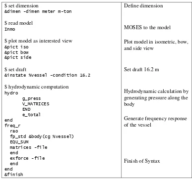
A schematic view of vessel modelling by panel model (meshed hull) to be used for 3D diffraction analysis is presented in Figure 3-18. Total panels generated is 977 panels, its see less number of panels due to the vessel shape is quite simple barge shape just like a box. The vessel have long parallel middle body and a simple stern shape plus skeg in stern. Bow part is a complex one to be modelled, therefore need a refine mesh or a lot of panels number in this area. Several degree of accuracy has been tried to obtain the accurate hydrodynamic result. In MOSES, author utilize a refine function to generate better mesh quality and can do easier work without a lot of time consuming require. A simple syntax of MOSES command input file is presented below in Table 3-6.
34
The second one is current. The current force on the vessel will be modelled as a static force. Only surface current will be utilized to define the current speed in below the water line. The effect of current on the wave drift forces and damping will also be taken into account.
The third is wave/swell. Both wave wind-driven sea and swell will be modelled using the following generalized, five-parameter JONSWAP wave spectrum:
S(f) = Hs2 Tp-4 f -5exp [ -1.25(Tp f)-4] γ exp[-(Tp^f-1)^2/2σ^2]
S(f) : Spectral wave energy distribution (m2/Hz)
Hs : Significant wave height (m)
35
3.2.6 Heading Analysis Algorithm
As stated by (T. Terashima, 2011), the set in heading angle is subject to external forces as show in equation below. Which is described as steady component of azimuth moment induced by wind, current, and wave (two wind waves and swell components) at turret position.
j : number wave and swell, where j=1:easterly wave, =2:westernly wave, =3:swell
w, c, ws (j) : incident angle of wind, current, and wave/swell where head is
defined zero
Lm : distance from turret position to the midship S (,j) : frequency spectrum of incident wave/swell G (θ,j) : directional distribution of incident wave/swell
Another author in (Morandini, 2007) also stated the algorithm regarding heading analysis. The slow drift loads are divided from the diagonal terms of the Quadratic Transfer Functions (QTFs) of the unit. The slow drift loads are computed based on Newman’s approximation. The formula used, however, involve four summations instead of two in the original formulation.
FD(t) is the one of three components in vessel axis system of slow drift loads at instant t, i.e. FDx, FDy, or MDψ
36
H is the wave incident relative to the vessel heading at instant t, i.e. H = H –ψ
QTF (H,K,K) is the relevant diagonal function interpolated for the instantaneous wave incident H.
sign(u) is equal to: 1 if u>0, -1 if u<0, 0 if u=0
The average value of FD(t) on the whole duration of simulation can be obtained by following equation.
FDmean = 2 ∫ 𝑄𝑇𝐹(𝛼𝐻,𝑚𝑀 ,)𝑆()𝑑
3.2.7 Heading Angles Calculation
The metocean reports provide the input environmental data for heading analysis. The mean vessel heading is determined for each sea-state. The long-term heading probability is used to determine extreme loads.
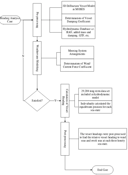
Figure 3-19 Heading Analysis Calculation Procedure
The environmental data includes a total of approximately 29,208 continuous three hourly hindcast sea states which represents 10 years of data. The environmental data includes:
Wind wave JONSWAP spectrum parameters (i.e. Hs, Tp, γ, σa and σb) and direction. (Two wave components for our cases i.e. westerly and easterly wave) Swell wave JONSWAP spectrum parameters (i.e. Hs, Tp, γ, σa and σb) and
direction. (Westerly swell for our cases) Wind mean speed and direction.
37
Figure 3-19 is presented simple procedure of heading analysis calculation. It was good to breaking down the methodology, as presented in Figure 3-21, to determine heading calculation in detail for a better understanding which starting from gather the vessel information and finish in obtaining a vessel long-term response in long-term metocean data set. The hydrodynamic database and the motion response in specific sea environment is presented in section 4.2.1 through 4.2.4. Furthermore the long-term response is presented in section 4.2.5. The procedure, which is adopted to (Sarala Resmi, 2011), is as follow:
1. A 3-D diffraction model of the vessel's hull was generated in MOSES based on the characteristics defined.
2. The calculated linearized roll damping is verified against field measurements and included in the hydrodynamic model.
3. A hydrodynamic database containing amplitude and phase of the RAOs for design parameters was prepared for frequency range of 0.1 rad/s to 1.5 rad/s with 0.05 rad/s increments and heading range of 0° to 360° with 22.5° increments.
4. The mooring arrangements were added to the MOSES model to perform static frequency domain simulation.
5. Wind and current coefficients from wind tunnel tests were added to the MOSES to include the wind drag and the current drag forces for the specified loading condition of the vessel and the headings relative to wind and current directions.
6. The three hourly environmental data, which contained sets of wind-sea, swell, wind and current data with their associated directions were included in the hydrodynamic model.
7. Using the MOSES software, the stable equilibrium positions for each three hourly sea state was calculated individually.
8. The vessel headings were post-processed to find the relative vessel heading to wind seas and swell seas at each three hourly sea state.
38
the moment is zero until and find a stable equilibrium position. Those condition is represent transient stage an steady stage in dynamic time domain simulation.
Figure 3-20 Equilibrium Calculation
From above two algorithms that stated by previous author in Section 3.2.5 the important point is an angle where the moment at the turret position is zero or near to zero, gives the balance heading angle of the vessel. Because the behavior of turret is free from moment that showing weathervaning effect. Balance heading will calculate for each environment condition as stated in Section 3.1, totally 29,208 cases.
In this thesis author will perform heading angles analysis by combination of software package MOSES and additional algorithm inside the syntax. The additional algorithm was generated to obtain estimation of heading angles position due to external load from environment to find zero moment at turret position. After the estimation value is obtained, an equilibrium command that already available in MOSES command is apply inside the syntax. A guess yaw angles algorithm are composed by following step:
1. Initialize stage. In this initial position, vessel force and moment due to external load is generated. Moment at the turret for this initial position shall be not have zero value.
2. Make a change position. To guess final yaw angle position, a delta angle is specified inside the algorithm. A determined increment angles shall set to estimated excursion each step and also get the force and moment at the changed position.
3. New state position. After delta angle was determined a new state position is obtained. In this new position the program will generate force and moment of the vessel and also new excursion position and the yaw angle.
39
4. Compute change until moment at turret 0. If moment at turret already captured the zero or near to zero value, heading angles is already obtained. But if those to find the relative vessel heading to wind seas and swell seas at each three hourly
sea state. Y
40
A sample of logging process of heading angles calculation is presented in Table 3-7.
Table 3-7 A Sample Logging File to Estimate Heading Angles
41
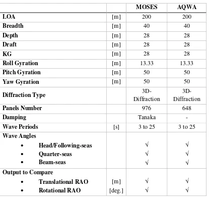
3.3 Model Verification
It should be note that this thesis will carried on by utilizing MOSES software package. Prior to do analyzing for all loadcases, a simple model will be verified between MOSES and another codes that have a similar capabilities for computing wave loads and motions of offshore structure in waves. The MOSES model will be verified against AQWA to compare the hydrodynamic result for a same simple model in a difference tools. AQWA is one of a well proven computer program that widely used for scientific and engineering practice purpose.
42
3.4 Assessing the Outcome
43
3.5 Mooring System Design
The global analysis of the coupled Vessel-Lines system will be performed with several software packages and numerical tools, both in the time-domain and frequency-domain. The methodology presented in Figure 3-22 and software tools that will be employed for the global analyses have been extensively verified by model tests for other deep water turret moored vessels. For diffraction analysis, the diffraction program MOSES will be used to provide an accurate representation of the vessel wave-frequency response. This thesis will study an optimum mooring design layout by considering heading analysis result.
3.5.1 Mooring System Characteristic
The mooring system is to be designed as permanent external turret. The mooring system consist of 12 mooring legs split into three (3) groups of four (4) legs (3by4 system). The separation each group is 120deg. However, another thing is the Centre to Centre anchor pile clearance shall enough to minimize interaction between two adjacent anchors. The optimum separation angle (°) between the mooring legs within a group will investigate in this thesis, which is required a clearance between adjacent mooring legs of two groups shall no less than 90deg as can be seen in Figure 3-23.
Turret Center is located 40m forward of the Fore Perpendicular (FP), 33m above keel. Determination of turret location and elevation shall consider mooring system performance, enough clearance of mooring to touch vessel bow in extreme condition, and also prevent green water impact. General 3D view of mooring system are presented in Figure 3-24.
3.5.2 Mooring Leg Components
44
Ropes. Mooring leg components and its properties is presented in Table 3-9, while mooring leg length is presented in Table 3-10.
Figure 3-22 External Turret Mooring System Design
45
Top Chain 157mm Grade R4 Studless Chain 2163.04 0.4943
Steel Wire 131mm Spiral Strand sheated steel wire 1884.66 0.0688
Bottom Chain 170mm Grade R3 Studless Chain 2536.08 0.5796
Table 3-10 Mooring Leg Lengths
46
Figure 3-23 Chain Table Layout
3.5.3 Marine Growth and Corrosion
Marine growth essentially increases the drag diameter of the component and also increases the unit weight of the component. To account for the marine growth effects, the drag diameter should be increased to the diameter of the component plus the marine growth thickness. The unit weight of the component should also be adjusted for the marine growth.
Chain corrosion have a potential for increased in corrosion in the splash zone, wear allowance of it is 0.8mm/year. The lower chain and ground chain have a normal corrosion allowance of 0.4mm/year. All chain shall be manufactured, inspected, and tested in accordance with test the latest API Specification 2F Specification for Mooring Chain, and DNV Certification Notes No. 2.6 (1995).
47
Figure 3-24 Schematic View of Mooring System
48
3.5.4 Environmental Condition
Long term environment data was already describe at Section 3.1, which is the set of data are will be utilize for fatigue analysis of mooring system. For mooring strength performance the cyclonic environment data with specified return period is needed. Here is return period of 10-yr for mooring design performance check and 200-yr for extreme condition. The parameters of Omni-directional cyclonic environmental conditions with 10-yr and 200-10-yr RPs are reflected in Table 3-11 and Table 3-12m respectively. The environmental modelling will remain same as Section 3.2.5.
Table 3-11 10-yr Return Period Environment Omni-Directional
Parameter Unit 10-yr wave, 10-yr wind,
and 10-yr current
Wave
Significant wave height (m) 4.74
Spectral peak period (s) 8.83
Jonswap peakedness parameter γ 1.24
Wind
1-hour mean speed (knots) 33.12
Current
Surface current speed (m/s) 0.74
Table 3-12 200-yr Return Period Environment Omni-Directional
Parameter Unit 200-yr wave, 200-yr wind,
and 200-yr current
Wave
Significant wave height (m) 7.28
Spectral peak period (s) 10.74
Jonswap peakedness parameter γ 1.36
Wind
1-hour mean speed (knots) 47.37
Current
49
3.5.5 Analysis Matrix and Load Cases
The following limit states will be considered for analysis and design of the mooring system.
1. Fatigue limit state: long-term operational environmental condition with intact mooring system.
2. Ultimate limit state: 200-yr Return Period environmental with intact mooring system.
3. Accidental limit state: 200-yr Return Period environmental with one-line-damaged mooring system.
Long-term environmental data has been available as per Section 3.1, contains 29,208 data simultaneously combination of 1-hour mean wind speed, surface current speed, and wave/swell. This data set will be utilized for mooring system fatigue analysis. The fatigue damage will be calculated using DNV formulation “Accumulated Fatigue Damage” that stated in DNV-OS-E301 Position Mooring Section 2 F 100 (DNV, 2010).
A spectral approach requires a more comprehensive description of the environmental data and loads, and a more detailed knowledge of these phenomena. Using the spectral approach, the dynamic effects and irregularity of the waves may be more properly accounted for. This approach involves the following steps:
1. Selection of major wave directions,
2. For each wave direction, select a number of sea states and the associated duration, which adequately describe the long-term distribution of the wave,
3. For each sea state, calculate the short-term distribution of stress ranges using a spectral method.
Combine the results for all sea states in order to derive the long-term distribution of stress range. In the following, a formulation is used to further illustrate below.
Fatigue assessment approach by DNV is in line with the MOSES methodology to assess the fatigue damage (Nachlinger, 1989). The assessment of fatigue is normally expressed by a cumulative damage ratio. In other words, by Miner's Rule
𝐶𝐷𝑅 =𝑇𝑡 ∫𝑁(𝑟) 𝑑𝑟𝑃(𝑟) ∞
0
where CDR is the cumulative damage ratio, T is the duration of a process, t is the average period for a stress cycle, P is the probability density function of the stress range,
50
and N is the average number of cycles to failure at a given stress range. Notice that if a body is subjected to several different sea states, then the total damage ratio can be obtained by adding the CDR's for each sea state.
Notice that the frequency domain is an ideal place to consider the fatigue problem. Once the deformation response operators have been computed, the stress spectrum (𝑆𝑠) is simply
𝑆𝑠 = |𝑆∗|2𝑆
where S* is the stress response operator and 𝑆
is the sea spectrum. Combine the results for all sea states in order to derive the long-term distribution of stress range. A wave scatter diagram has been used to describe the wave climate for fatigue damaged assessment. The wave scatter diagram is represented by the distribution of Hs and Tp. The environmental wave spectrum 𝑆 for the different sea states can be defined, i.e. applying the JONSWAP wave spectrum. Now, using the Raleigh distribution
𝑃(𝑟) =4𝑚𝑟
Thus, the cumulative damage is easily computed from the stress response operators. Mathematically, Spectral-based Fatigue Analysis begins after the determination of the stress transfer function. Wave data are then incorporated to produce stress-range response spectra, which are used to describe probabilistically the magnitude and frequency of occurrence of local stress ranges at the locations for which fatigue strength is to be calculated. Wave data are represented in terms of a wave scatter diagram and a wave energy spectrum. The wave scatter diagram consists of sea-states, which are shortterm descriptions of the sea in terms of joint probability of occurrence of a significant wave height, Hs, and a characteristic period.
An appropriate method is to be employed to establish the fatigue damage resulting from each considered sea state. The damage resulting from individual sea states is referred
to as “short-term”. The total fatigue damage resulting from combining the damage from
(3.6)
51
each of the short-term conditions can be accomplished by the use of a weighted linear summation technique (i.e., Miner’s Rule).
The total expected damage for all seastates during the life of the structure is the sum of the damages for each individual seastate. Cumulative fatigue damage effect calculations
are based on Miner’s rule of linear accumulation with the appropriate S-N curve. The
cumulative damage ratio (CDR), summed over all the various loads, shall not exceed 1.0. However, the Cumulative Damage Ratio (CDR) result computed by MOSES does not include the Design Fatigue Factors (DFF). Thus for corresponding targeted CDR is
𝐶𝐷𝑅 ≤𝐷𝐹𝐹1
The predicted fatigue life is then calculated as:
𝑃𝑟𝑒𝑑𝑖𝑐𝑡𝑒𝑑𝐹𝑎𝑡𝑖𝑔𝑢𝑒𝐿𝑖𝑓𝑒(𝑦𝑒𝑎𝑟𝑠) =𝐷𝑒𝑠𝑖𝑔𝑛𝑆𝑒𝑟𝑣𝑖𝑐𝑒𝐿𝑖𝑓𝑒𝐶𝐷𝑅
Moreover, Design Performance Limit State (10-yr RP environment) will not be included in this study as the extreme condition should be enough for ensure the reliable and efficient mooring system in term of mooring loads and vessel offsets for the riser design. The load cases for ultimate limit state and accidental limit state are defined using Omni-directional environment information as per Section 3.5.4 with 15deg resolution covering the entire 360deg. A number of environment alignment cases were created based on the DNV POSMOOR guidelines where the wind direction is modified up to a maximum of 30 degrees off the wave direction and the current up to a maximum of 45 degrees on the same side of the waves. The following combinations were used for the mooring analysis:
1. C1 - Collinear: Wind, wave and current from the same direction (aligned) 2. C2 - Crossed 1: Wind and current 30 degrees off the wave direction.
3. C3 - Crossed 2: Wind at 30 degrees off the waves, and current 45 degrees off the waves (on the same side as the wind).
Tension ratio is need to be considered at design of mooring configuration. Maximum tension should be limited by the tension ratio. It is defined as follow:
𝑇𝑒𝑛𝑠𝑖𝑜𝑛𝑅𝑎𝑡𝑖𝑜 = 𝑀𝑖𝑛𝑖𝑚𝑢𝑚𝐵𝑟𝑒𝑎𝑘𝑖𝑛𝑔𝐿𝑜𝑎𝑑𝐴𝑝𝑝𝑙𝑖𝑒𝑑𝑇𝑒𝑛𝑠𝑖𝑜𝑛
(3.8)
(3.9)
52 30*10 = 300-yr fatigue life) as specified by ABS Rules for Classing and Building Floating Production Installations. (ABS, 2009)
2. Maximum ratio of maximum tension and breaking tension on anchor leg for an intact mooring system must be lower than 0.6 based on dynamic simulation. 3. Maximum ratio of maximum tension and breaking tension on anchor leg for a
one-line-damage mooring system must be lower than 0.8 based on dynamic simulation. 4. Maximum vessel offsets for both intact and damaged mooring system must be
restricted in consideration of riser system integrity (if any).
Allowable maximum tension and vessel offsets are presented in below:
Table 3-13 Mooring System Design Criteria
Limit State Mooring System Maximum
Tension Ratio conditions for intact or damaged mooring system.
6. No interference between anchor legs and risers under any design storm conditions for intact or damaged mooring system.