Risk Based Inspection (RBI) of Gas Cooling Heat Exchanger - ITS Repository

(1)

BACHELOR THESIS – ME 141502

Risk Based Inspection (RBI) Of Gas-Cooling Heat Exchanger

Alfa Muhammad Megawan NRP. 4213101020

Supervisor:

Ir. Dwi Priyanta, M.SE.

Co-Supervisor:

Nurhadi Siswantoro, ST., MT.

DOUBLE DEGREE PROGRAM OF MARINE ENGINEERING DEPARTMENT Faculty of Marine Technology

Institut Teknologi Sepuluh Nopember Surabaya

(2)

(3)

(4)

SKRIPSI – ME 141502

Analisa Penjadwalan Inspeksi pada Heat Exchanger Pendingin Gas dengan Menggunakan Metode Inspeksi Bedasarkan Analisa Risiko

Alfa Muhammad Megawan NRP. 4213 101 020

Dosen Pembimbing 1: Ir. Dwi Priyanta, M.SE

Dosen Pembimbing 2: Nurhadi Siswantoro, ST., MT.

PROGRAM DOUBLE DEGREE

DEPARTEMEN TEKNIK SISTEM PERKAPALAN Fakultas Teknologi Kelautan

Institut Teknologi Sepuluh Nopember Surabaya

(5)

(6)

(7)

i

APPROVAL FORM

RISK BASED INSPECTION (RBI) OF GAS-COOLING HEAT EXCHANGER

BACHELOR THESIS

Submitted to Comply One of The Requirement to Obtain a Bachelor of Engineering

on

Marine Operation and Maintenance (MOM) Department of Marine Engineering

Faculty of Marine Technology Institut Teknologi Sepuluh Nopember

Prepared by:

ALFA MUHAMMAD MEGAWAN NRP. 4213101020

Approved by Supervisor and Co-Supervisor: 

1. Ir. Dwi Priyanta, M.SE. ( )

(8)

ii

(9)

iii

APPROVAL FORM

BACHELOR THESIS

on

Prepared by:

Approved by

Head of Marine Engineering Departement

(10)

iv

(11)

v

APPROVAL FORM

BACHELOR THESIS

on

Prepared by:

Approved by

Representative of Hochschule Wismar in Indonesia

(12)

vi

(13)

vii

DECLARATION OF HONOR

I hereby who signed below declare that:

This final project has written and developed independently without any plagiarism act. All contents and ideas drawn directly from internal and external sources are indicated such as cited sources, literatures, and other professional sources.

Name : Alfa Muhammad Megawan

ID Number : 4213101020

Final Project Title : Risk Based Inspection (RBI) of Gas-Cooling Heat Exchanger

Department : Marine Engineering

If there is plagiarism act in the future, I will fully responsible and receive the penalty given by ITS according to the regulation applied.

Surabaya, July 2017

(14)

viii

(15)

ix

Risk Based Inspection (RBI) of Gas-Cooling Heat Exchanger

Name : Alfa Muhammad Megawan

NRP : 4213101020

Department : Double Degree Program of Marine Engineering Supervisor : Ir. Dwi Priyanta, M.SE.

Co-Supervisor : Nurhadi Siswantoro, ST., MT.

ABSTRACT

On October 2013, Pertamina Hulu Energi Offshore North West Java (PHE – ONWJ) platform personnel found 93 leaking tubes locations in the finfan coolers/ gas-cooling heat exchanger. After analysis had been performed, the crack in the tube strongly indicate that stress corrosion cracking was occurred by chloride. Chloride stress corrosion cracking (CLSCC) is the cracking occurred by the combined influence of tensile stress and a corrosive environment. CLSCC is the one of the most common reasons why austenitic stainless steel pipework or tube and vessels deteriorate in the chemical processing, petrochemical industries and maritime industries. In this thesis purpose to determine the appropriate inspection planning for two main items (tubes and header box) in the gas-cooling heat exchanger using risk based inspection (RBI) method. The result, inspection of the tubes must be performed on July 6, 2024 and for the header box inspection must be performed on July 6, 2025. In the end, RBI method can be applicated to gas-cooling heat exchanger. Because, risk on the tubes can be reduced from 4.537 m2_{/year to 0.453 m}2_{/year. And inspection planning for header box can be reduced}

(16)

x

(17)

xi

Analisa Penjadwalan Inspeksi pada Heat Exchanger Pendingin Gas dengan Menggunakan Metode Inspeksi Bedasarkan Analisa Risiko

Nama : Alfa Muhammad Megawan

NRP : 4213101020

Departemen : Teknik Sistem Perkapalan Program Double Degree

Dosen Pembimbing 1 : Ir. Dwi Priyanta, M.SE.

Dosen Pembimbing 2 : Nurhadi Siswantoro, ST., MT.

ABSTRAK

(18)

xii

(19)

xiii

PREFACE

Alhamdulillahirobbil ‘alamin. Praise is merely to the Almighty Allah SWT for the gracious mercy and tremendous blessing which enables the author to accomplish this bachelor thesis.

This thesis report entitled: ”Risk Based Inspection (RBI) of Gas-Cooling Heat Exchanger” is submitted to fulfill one of the requirements in accomplishing the bachelor degree program at Marine Engineering Department, Faculty of Marine Technology, Institut Teknologi Sepuluh Nopember Surabaya. Conducting this research study is not possible without all helps and supports from various parties. Therefore, the author would like to thank to all people who has support the author for accomplishing this bachelor thesis, among others:

1. Mr. Dr. Eng. Muhammad Badrus Zaman, ST., MT. as the Head of Marine Engineering Department.

2. Mr. Prof. Semin, ST., MT., Ph.D as the Secretary of Marine Engineering Department.

3. Mr. Dr. I Made Ariana, ST., MT. as Author’s Lecturer Advisor since first semester until eighth semester.

4. Mr. Ir. Dwi Priyanta, M.SE. as Author’s Thesis Supervisor and Secretary of Double Degree Program in Marine Engineering Department who has giving the ideas, correction, and guidance during the thesis is conducted.

5. Mr. Nurhadi Siswantoro, ST., MT. as Author’s Thesis Co-Supervisor who has giving the motivation and every necessary information to help finish the bachelor thesis.

6. Irfan Syarif Arief, ST., MT. as the head of MMD Laboratory who has giving permission to do any activities inside the lab and provides place during the working of bachelor thesis.

7. To my parents, Mr Firmansyah, Mrs. Yuyun Suniarti and also my lovely brother who always give their loves, prayers, supports, and encouragements for every single path the author chooses.

8. Muthya Shinta Devi, S.Ked who always be author’s loyal supporter in every conditions.

(20)

xiv

10.Mr Apri Densi and Mr Indarta Muhammad and All of PHE ONWJ Mechanical and Piping Team for giving any data required for this thesis.

11.BARAKUDA ’13 and Marine Double Degree ’13 for the assistance and support.

12.Great amounts of friends that can’t be mentioned, for their support, help and ideas for this thesis.

The author realizes that this thesis remains far away from perfect. Therefore, every constructive suggestion and idea from all parties is highly expected by author for this bachelor thesis correction and improvement in the future.

Finally, may Allah SWT bestow His grace, contentment and blessings to all of us. Hopefully, this bachelor thesis can be advantageous for all of us particularly for the readers.

Surabaya, July 2017

(21)

xv

2.2.1.3.2.1.4. Calculation Procedure of Estimate the Fluid Inventory Available for Release (Available Mass) ... 25 2.2.1.3.2.1.5. Calculation Procedure of Determining the Release Type (Continuous or Instantaneous) ... 27 2.2.1.3.2.1.6. Estimate the Impact of Detection and Isolation Systems on Release Magnitude ... 27 2.2.1.3.2.1.7. Determining the Release Rate and Mass for Consequence Analysis ... 29 2.2.1.3.2.1.8. Flammable and Explosive Consequence ... 29 2.2.1.3.2.2. Level 2 Consequence Analysis ... 35 2.2.1.4. Remaining Lifetime Analysis ... 36 CHAPTER 3 ... 37 METHODOLOGY ... 37 3.1. Literatures Study ... 38 3.2. Determine Generic Failure Frequency ... 38 3.3. Determining Damage Mechanism ... 38 3.4. Final Damage Factor Calculation ... 38 CHAPTER 4 ... 39 DATA ANALYSIS ... 39 4.1. Collecting Asset Data ... 39 4.2. Generic Failure Frequency (gff) ... 40 4.3. Damage Mechanism Identification... 40 4.3.1. Calculation of Thinning Damage Factor ... 42 4.3.2. Calculation of CL-SCC Damage Factor... 46 4.3.3. Total Damage Factor ... 47 4.4. Calculation of Consequence ... 48 4.4.1. Determining the Representative Fluid and Associated Properties 48 4.4.2. Release Hole Size Selection... 49 4.4.3. Release Rate Calculation ... 49 4.4.4. Estimate the Fluid Inventory Available for Release (Available Mass) ... 50 4.4.5. Determining the Release Type (Continuous or Instantaneous) ... 51 4.4.6. Estimate the Impact of Detection and Isolation Systems on Release

(23)

xvii

(24)

xviii

(25)

xix

LIST OF TABLES

Table 2.1 Suggested Component Generic Failure Frequencies (gff) ... 9 Table 2.2 damage factor defined ... 13 Table 2.3 Inspection Effectiveness Categories ... 14 Table 2.4 Management Systems Evaluation ... 15 Table 2.5 Susceptibility to Cracking – CLSCC ... 19 Table 2.6 Determination of Severity Index – CLSCC ... 19 Table 2.7 SCC Damage Factors – All SCC Mechanisms ... 19 Table 2.8 List of Representative Fluids Available for Level 1 Analysis ... 22 Table 2.9 Properties of the Representative Fluids Used in Level 1 Analysis ... 23 Table 2.10 Consequence Analysis Guidelines for Determining the Phase of a Fluid ... 24 Table 2.11 Release Hole Sizes and Area used ... 24 Table 2.12 Assumption When Calculating Liquid Inventories Within Equipment ... 25 Table 2.13 Detection and Isolation System Rating Guide ... 27 Table 2.14 Adjustments to Release Based on Detection and Isolation Systems . 28 Table 2.15 Leak Durations Based on Detection and Isolation Systems ... 28 Table 2.16 Adjustments to Flammable Consequences for Mitigation Systems ... 30 Table 2.17 Component Damage Flammable Consequence Equation Constants 31 Table 4.1 Asset specification data ... 39 Table 4.2 Determine the generic failure frequency from table. ... 40 Table 4.3 damage mechanism identification ... 41 Table 4.4 Guidelines for Assigning Inspection Effectiveness – General Thinning ... 43 Table 4.5 Guidelines for Assigning Inspection Effectiveness – Local Thinning .... 43 Table 4.6 basic damage factor determining for tube in RBI date ... 45 Table 4.7 Susceptibility to Cracking – CLSCC ... 46 Table 4.8 Determination of Severity Index – CLSCC ... 46 Table 4.9 Based SCC Damage Factors (red square is for the header box and blue square is for the tube)... 47 Table 4.10 Summary of release hole size area... 49 Table 4.11 Summary of release hole size area... 49 Table 4.12 Summary of fluid mass calculation (massadd,n) ... 50

Table 4.13 Summary of available mass for release (massavail,n) ... 50

(26)

xx

(27)

xxi

LIST OF FIGURES

(28)

xxii

(29)

1

CHAPTER 1 INTRODUCTION

1.1. Overview

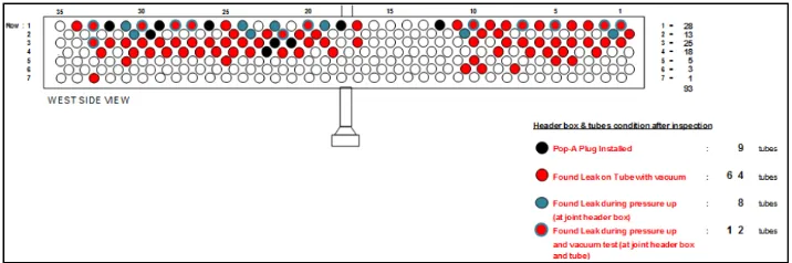
On October, 2013, Pertamina Hulu Energi Offshore North West Java (PHE – ONWJ) platform personnel found 93 leaking tubes reported in gas cooling heat exchanger (figure 1.1) on the one of Pertamina platform. This situation made the gas cooling heat exchanger not in a good performance. For the forward PHE-ONWJ need effective maintenance strategy for oil and gas platform equipment especially for gas cooling heat exchanger.

Figure 1.1 Gas-cooling heat exchanger leakage report (Company report, 2013)1

According to the function of heat exchangers, there are view types of heat exchangers used in oil and gas facility, they are; shell and tube, double pipe, plate and frame, aerial cooler, bath type, forced air, and direct fired. (Arnold & Stewart, 1989)

Based on the explanation above, Pertamina PHE-ONWJ gas cooling heat exchanger classified as areal cooler heat exchanger because its function is cooling the gas with a fan in to near ambient temperature.

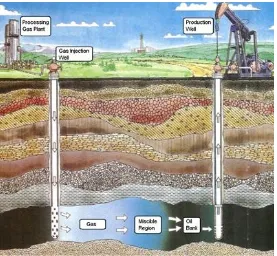
Heat exchanger is the one of crucial equipment in the processing facility especially in the oil and gas industry sector. Heat exchanger is used to transfer heat between one and more fluids. Ones of heat exchanger application is for cooling the gas before injected to the oil reservoir. Gas injection is the method to increase oil production by boosting depleted pressure in the reservoir (figure 1.2). Another function of gas cooling heat

(30)

exchanger is for cooling the gas before supply the gas turbine to generated electric power on the platform.

Figure 1.2 optimization oil production by gas injection method 2

American Petroleum Institute (API) is the one of the most widely used standard guideline in oil and gas company around the world besides DNV-GL. PHE-ONWJ as an Indonesian national oil and gas company install API standard for their company equipment. For the example PHE-ONWJ platform adopt guidelines from API 660 and API 661 for gas cooling heat exchanger fabrication and installation.

One of maintenance strategies for gas cooling heat exchanger can be developed by using Risk Based Inspection (RBI). by using RBI company will get information using risk analysis to develop an effective inspection plan. Identification of company equipment is the beginning of the systematic process in the inspection planning. Probability of failure and consequence of failure are the basic formula to calculate the RBI and must be evaluated by considering all damage mechanism directly effect to the equipment or

(31)

3

the system. However, failure scenarios according to the actual damage mechanism should be develop and considered.

RBI methodology produces optimal inspection planning for the asset and make the priority from the lower risk to the higher risk. In other word inspection planning in RBI focused to identification what to inspect, how to inspect, where to inspect and how often to inspect. Inspection planning used to control degradation of the asset and the company will get considerable impact in the system operation and the appropriate economic consequences. (Faber, 2001)

1.2. Problems

According to the overview above the main problems of thesis are:

1. How to determine damage factor for the gas cooling heat exchanger based on RBI method?

2. How to determine the risk level for the gas cooling heat exchanger based on RBI method?

3. How to determine appropriate inspection planning with the gas cooling heat exchanger condition?

4. How to determine the remaining useful life according to the risk level of the gas cooling heat exchanger?

1.3. Limitations

The limitations of the thesis are:

1. Gas cooling heat exchanger which is the object of study belong to PHE-ONWJ.

2. All of the study and calculation based on API 581. 3. Natural disasters are not taken into consideration.

1.4. Objectives

The objectives of this thesis are:

1. Determine damage factor of gas cooled heat exchanger according to RBI method.

2. Determine risk level of gas cooling heat exchanger.

3. Determine remaining life according to the gas cooling heat exchanger risk level.

(32)

1.5. Benefits

The benefits of the thesis are:

1. This thesis can be company consideration materials to determine priority of the maintenance and inspection strategy as a preventive effort to minimalized the failure.

2. Introduce RBI as a maintenance and inspection strategy based on risk analyze of the pressure vessel.

(33)

5

CHAPTER 2 LITERATURE STUDY

2.1. Asset Overview

2.1.1. Gas Cooling Heat Exchanger 2.1.1.1. Operating Principal

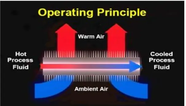
As shown in figure (2.1), Gas cooling heat exchangers or aerial coolers are often used to cooling a hot fluid to near ambient temperature. They are mechanically simple and flexible. They eliminate the nuisance and cost of a cold source. In warm climates, aerial coolers may not be capable of providing as low a temperature as shell-and-tube heat exchangers, which use a cool medium. In aerial coolers, the tube bundle is on the discharge or suction side of a fan, depending on whether the fan is blowing air across the tubes or sucking air through them. This type of exchanger can be used to cool a hot fluid to something near ambient temperature as in a compressor inter stage cooler, or it can be used to heat the air as in a space heater.

Figure 2.1 gas cooling heat exchanger operation principle3

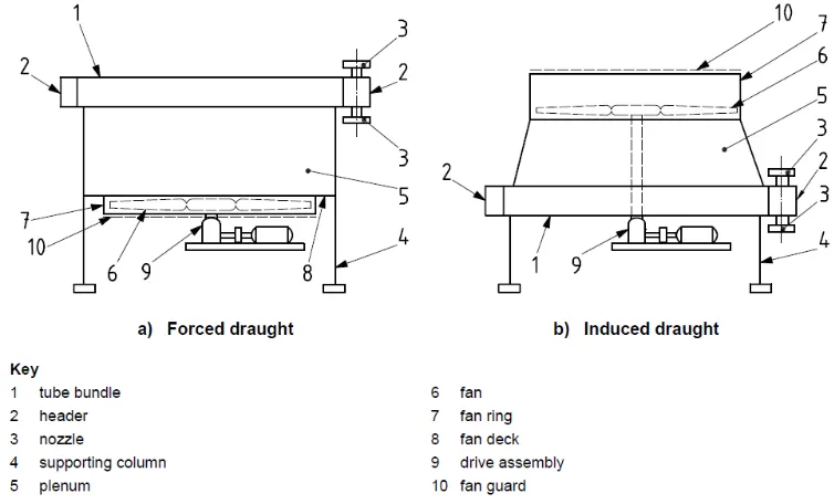
2.1.1.2. Type of Gas-Cooling Heat Exchanger

When the tube bundle is on the discharge of the fan, the exchanger is referred to as “forced draft” (Figure 2.2). When the tube bundle is on the suction of the fan it is referred to as an “induced draft” exchanger (Figure 2.2).In figure 2.2 the process fluid enters one of the nozzles on

(34)

the fixed end and the pass partition plate forces it to flow through the tubes to the floating end (tie plate). Here it crosses over to the remainder of the tubes and flows back to the fixed end and out the other nozzle. Air is blown vertically across the finned section to cool the process fluid. Plugs are provided opposite each tube on both ends so that the tubes can be cleaned or individually plugged if they develop leaks, tube bundle could also be mounted in a vertical plane, in which case air would be blown horizontally through the cooler.

Figure 2.2 Structure of gas cooling heat exchanger (API 661, 2006)

2.1.1.3. Structure of Gas Cooling Heat Exchanger

(35)

7

2.2. Method Overview

2.2.1. Risk Based Inspection (RBI)

Inspection can be interpreted as planning, implementation and evaluation of examinations to determine physical and metallurgical condition of equipment during the performance of good service. Examination methods including visual surveys and nondestructive test techniques, such as ultrasonic inspection magnetic particle inspection, radiographic inspection and so on, design to detect and calculate wall thinning and defects.

The information of inspection planning in risk based inspection based on the risk analysis of the equipment. The purpose of the risk analysis is to identify the potential degradation mechanisms and threats to the integrity of the equipment and to assess the consequences and risk of failure. (J B Wintle & G J Amphlett, 2001)

2.2.1.1. Risk

Risk is defined as the combination probability of asset failure and consequence if the failure happened. Risk can be expressed numerically with formula (2.1) as shown below.

Risk = Probability x Consequence (2.1)

2.2.1.2. Probability of Failure

The probability of failure may be determined based on one, or a combination of the following methods:

a) Structural reliability models – In this method, a limit state is defined based on a structural model that includes all relevant damage mechanisms, and uncertainties in the independent variables of this models are defined in terms of statistical distributions. The resulting model is solved directly for the probability of failure.

b) Statistical models based on generic data – In this method, generic data is obtained for the component and damage mechanism under evaluation and a statistical model is used to evaluate the probability of failure.

(36)

In API RBI, a combination of the above is used to evaluate the probability of failure in terms of a generic failure frequency and damage factor. The probability of failure calculation is obtained from the equation (2.2).

Pof (t) = gff x Df (t) x FMS (2.2)

Where:

gff = generic failure frequency Df (t) = damage factor

FMS = management system factor

2.2.1.2.1. Generic Failure Frequency (gff)

The generic failure frequency can be determined by industry average of asset failure. The generic failure frequency is expected to the previous failure frequency to any specific damage happening from exposure to the operating environment. There are four different damage hole sizes model the release scenarios covering a full range of events they are small, medium, large, and rupture.

If the data of the asset is complete, actual probabilities of the failure could be calculated with actual observed failures. Even if a failure has not occurred in a component, the true probability of failure is likely to be greater than zero because the component may not have operated long enough to experience a failure. As a first step in estimating this non-zero probability, it is necessary to examine a larger set of data of similar components to find enough failures such that a reasonable estimate of a true probability of failure can be made.

(37)

9

The generic failure frequency is intended to be the failure frequency representative of failures due to degradation from relatively benign service prior to accounting for any specific operating environment, and are provided for several discrete hole sizes for various types of processing equipment (i.e. process vessels, drums, towers, piping systems, tankage, etc.).

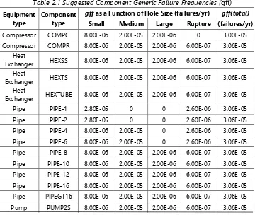
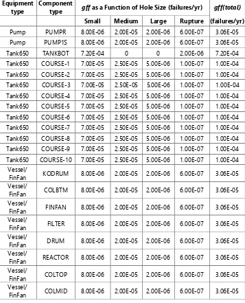
A recommended list of generic failure frequencies is provided in table (2.1) The generic failure frequencies are assumed to follow a log-normal distribution, with error rates ranging from 3% to 10%. Median values are given in table (2.1) The data presented in the table (2.1) is based on the best available sources and the experience of the API RBI Sponsor Group.

The overall generic failure frequency for each component type was divided across the relevant hole sizes, i.e. the sum of the generic failure frequency for each hole size is equal to the total generic failure frequency for the component.

Table 2.1 Suggested Component Generic Failure Frequencies (gff)

Equipment type

Component type

gff as a Function of Hole Size (failures/yr) gff(total)

Small Medium Large Rupture (failures/yr)

Compressor COMPC 8.00E-06 2.00E-05 2.00E-06 0 3.00E-05

Compressor COMPR 8.00E-06 2.00E-05 2.00E-06 6.00E-07 3.06E-05

Heat

Exchanger HEXSS 8.00E-06 2.00E-05 2.00E-06 6.00E-07 3.06E-05

Heat

Exchanger HEXTS 8.00E-06 2.00E-05 2.00E-06 6.00E-07 3.06E-05

Heat

Exchanger HEXTUBE 8.00E-06 2.00E-05 2.00E-06 6.00E-07 3.06E-05

Pipe PIPE-1 2.80E-05 0 0 2.60E-06 3.06E-05

Pipe PIPEGT16 8.00E-06 2.00E-05 2.00E-06 6.00E-07 3.06E-05

(38)

Table 2.1 Suggested Component Generic Failure Frequencies (gff) (Continue) Equipment

type

Component

type gff as a Function of Hole Size (failures/yr) gff(total)

Small Medium Large Rupture (failures/yr)

Pump PUMPR 8.00E-06 2.00E-05 2.00E-06 6.00E-07 3.06E-05

Pump PUMP1S 8.00E-06 2.00E-05 2.00E-06 6.00E-07 3.06E-05

Tank650 TANKBOT 7.20E-04 0 0 2.00E-06 7.20E-04

Tank650 COURSE-1 7.00E-05 2.50E-05 5.00E-06 1.00E-07 1.00E-04

Vessel/

FinFan KODRUM 8.00E-06 2.00E-05 2.00E-06 6.00E-07 3.06E-05

Vessel/

FinFan COLBTM 8.00E-06 2.00E-05 2.00E-06 6.00E-07 3.06E-05

Vessel/

FinFan FINFAN 8.00E-06 2.00E-05 2.00E-06 6.00E-07 3.06E-05

Vessel/

FinFan FILTER 8.00E-06 2.00E-05 2.00E-06 6.00E-07 3.06E-05

Vessel/

FinFan DRUM 8.00E-06 2.00E-05 2.00E-06 6.00E-07 3.06E-05

Vessel/

FinFan REACTOR 8.00E-06 2.00E-05 2.00E-06 6.00E-07 3.06E-05

Vessel/

FinFan COLTOP 8.00E-06 2.00E-05 2.00E-06 6.00E-07 3.06E-05

Vessel/

FinFan COLMID 8.00E-06 2.00E-05 2.00E-06 6.00E-07 3.06E-05

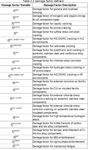
2.2.1.2.2. Damage Mechanism or Damage Factor

(39)

11

The basic function of the damage factor is to statistically evaluate the amount of damage that may be present as a function of time in service and the effectiveness of an inspection activity to quantify that damage.

Damage factor estimates are currently provided for the following damage mechanisms:

a) Thinning (general and local) - 𝑑_𝑓𝑡ℎ𝑖𝑛.

b) Component Linings - 𝑑_𝑓𝑒𝑙𝑖𝑛.

c) External Damage (corrosion and stress corrosion cracking) - 𝑑_𝑓𝑒𝑥𝑡𝑑.

d) Stress Corrosion Cracking (internal based on process fluid, operating conditions and materials of construction) - 𝑑_𝑓𝑆𝐶𝐶.

e) High Temperature Hydrogen Attack - 𝑑_𝑓ℎ𝑡ℎ𝑎.

f) Mechanical Fatigue (Piping Only) - 𝑑_𝑓𝑚𝑓𝑎𝑡.

g) Brittle Fracture (including low-temperature brittle fracture, temper

embrittlement, 885 embrittlement, and sigma phase

embrittlement.) - 𝑑_𝑓𝑏𝑟𝑖𝑡.

Damage factors are calculated based on the techniques described in probability of failure calculation method paragraph, but are not intended to reflect the actual probability of failure for the purposes of reliability analysis. Damage factors reflect a relative level of concern about the component based on the stated assumptions in each of the applicable paragraphs of the document.

If the damage factor has combination or multiple damage mechanism then the rules and the formulas are as follows:

a) Total damage factor, Df-total – If more than one damage mechanism

is present, the following rules are used to combine the damage factors. The total damage factor is given by equation (2.3) when the thinning is local:

Df-total = max[𝑑_{𝑓−𝑔𝑜𝑣}𝑡ℎ𝑖𝑛 , 𝑑_{𝑓−𝑔𝑜𝑣}e𝑥𝑡𝑑 ] + 𝑑_{𝑓−𝑔𝑜𝑣}𝑆𝐶𝐶 + 𝑑_{𝑓−𝑔𝑜𝑣}ℎ𝑡ℎ𝑎 + 𝑑_{𝑓−𝑔𝑜𝑣}𝑏𝑟𝑖𝑡 + 𝑑_{𝑓−𝑔𝑜𝑣}𝑚𝑓𝑎𝑡

(40)

Df-total = 𝑑_𝑓𝑡ℎ𝑖𝑛 + 𝑑_𝑓𝑒𝑥𝑡𝑑 + 𝑑_{𝑓−𝑔𝑜𝑣}𝑆𝐶𝐶 + 𝑑_{𝑓−𝑔𝑜𝑣}ℎ𝑡ℎ𝑎 + 𝑑_{𝑓−𝑔𝑜𝑣}𝑏𝑟𝑖𝑡 + 𝑑_{𝑓−𝑔𝑜𝑣}𝑚𝑓𝑎𝑡 (2.4)

*if a damage factor is less than or equal to one, then this damage factor shall be set to zero in the summation.

*if Df-total is computed as less than or equal to one, then Df-total shall

be set equal to one.

b) Governing Thinning Damage Factor, D_f−govthin – governing thinning damage factor is determined based on the presence of an internal liner using equations (2.5) and (2.6).

𝑑_{𝑓−𝑔𝑜𝑣}𝑡ℎ𝑖𝑛 _{= min [}_𝑑

𝑓𝑡ℎ𝑖𝑛, 𝑑𝑓𝑒𝑙𝑖𝑛] when an internal liner is present (2.5)

𝑑𝑓−𝑔𝑜𝑣𝑡ℎ𝑖𝑛 = 𝑑𝑓𝑡ℎ𝑖𝑛when an internal liner is not present (2.6)

c) Governing Stress Corrosion Cracking Damage Factor, 𝑑_{𝑓−𝑔𝑜𝑣}𝑆𝐶𝐶 – The governing stress corrosion cracking damage factor is determined from equation (2.7).

𝑑𝑓−𝑔𝑜𝑣𝑆𝐶𝐶 = max [𝑑𝑓𝑐𝑎𝑢𝑠𝑡𝑖𝑐, 𝑑𝑓𝑎𝑚𝑖𝑛𝑒, 𝑑𝑓𝑆𝐶𝐶, 𝑑_𝑓

𝐻𝐼𝐶

𝑆𝑂𝐻𝐼𝐶−𝐻2𝑆_,_𝑑

𝑓𝑐𝑎𝑟𝑏𝑜𝑛𝑎𝑡𝑒, 𝑑𝑓𝑃𝑇𝐻𝐴,

𝑑𝑓𝐶𝐿𝑆𝐶𝐶, 𝑑𝑓𝐻𝑆𝐶−𝐻𝐹, 𝑑𝑓

𝐻𝐼𝐶

𝑆𝑂𝐻𝐼𝐶− 𝐻𝐹_] _(2.7)

d) Governing External Damage Factor, d_f−govextd , governing external damage factor is determined fromequation (2.8).

𝑑𝑓−𝑔𝑜𝑣extd = max [ 𝑑𝑓𝑒𝑥𝑡𝑑, 𝑑𝑓𝐶𝑈𝐼𝐹, 𝑑𝑓𝑒𝑥𝑡𝑑−𝐶𝐿𝑆𝐶𝐶, 𝑑𝑓𝐶𝑈𝐼−𝐶𝐿𝑆𝐶𝐶] (2.8)

e) Governing Brittle Fracture Damage Factor, 𝑑_{𝑓−𝑔𝑣}𝑏𝑟𝑖𝑡 The governing brittle fracture damage factor is determined fromequation (2.9).

𝑑_{𝑓−𝑔𝑜𝑣}𝑏𝑟𝑖𝑡 _{= max [(}_𝑑

𝑓𝑏𝑟𝑖𝑡𝑓𝑟𝑎𝑐𝑡+𝑑𝑓𝑡empe), 𝑑𝑓885, 𝑑𝑓𝑠𝑖𝑔𝑚𝑎) (2.9)

(41)

13

Table 2.2 damage factor defined

Damage Factor Variable Damage Factor Description

𝑑𝑓𝑡ℎ𝑖𝑛 Damage factor for general and localized _thinning

𝐷𝑓𝑙𝑖𝑛𝑒𝑟 Damage factor of inorganic and organis linings _{for all component types}

𝐷𝑓`𝑐𝑎𝑢𝑠𝑡𝑖𝑐 Damage factor for caustic cracking

𝐷𝑓𝑎𝑚𝑖𝑛𝑒 Damage factor for amine cracking

𝐷𝑓𝑠𝑠𝑐 Damage factor for sulfide stress corrosion _cracking

𝐷𝑓𝐻𝐼𝐶−𝑆𝑂𝐻𝐼𝐶−𝐻2𝑆 Damage factor for HIC/SOHIC cracking in H_environments 2S

𝐷𝑓𝑐𝑎𝑟𝑏𝑜𝑛𝑎𝑡𝑒 Damage factor for carbonate cracking

𝐷𝑓𝑃𝑇𝐴

Damage factor for polythionic acid cracking in austenitic stainless steel and nonferrous alloy components

𝐷𝑓𝐶𝐿𝑆𝐶𝐶 Damage factor for chloride stress corrosion _cracking

𝐷𝑓𝐻𝑆𝐶−𝐻𝐹 Damage factor for hydrogen stress cracking in _{HF environment}

𝐷_𝑓HIC/SOHIC−HF Damage factor for HIC/SOHIC cracking in HF _environments 𝐷𝑓𝑒𝑥𝑡𝑜𝑟 Damage factor for external corrosion on ferritic _components

𝐷𝑓𝐶𝑈𝐼𝐹 Damage factor for CUI on insulted ferritic _components

𝐷𝑓𝑒𝑥𝑡−𝐶𝐿𝑆𝐶𝐶

Damage factor for external chloride stress corrosion cracking on austenitic stainless steel components

𝐷𝑓𝐶𝑈𝐼−𝐶𝐿𝑆𝐶𝐶

Damage factor for external chloride stress corrosion cracking on austenitic stainless steel insulated components

𝐷𝑓ℎ𝑡ℎ𝑎 Damage factor for high temperature hydrogen _attack

𝐷_𝑓𝑏𝑟𝑖𝑡𝑓𝑟𝑎𝑐𝑡 Damage factor for brittle fracture of carbon

steel and low alloy components

𝐷_𝑓𝑡𝑒𝑚𝑝𝑒 Damage factor for temper embrittlement of

Cr-Mo low alloy components

𝐷𝑓885 Damage factor for 885 embrittlement

𝐷𝑓𝑠𝑖𝑔𝑚𝑎 Damage factor for sigma phase embrittlement

𝐷_𝑓𝑚𝑓𝑎𝑡 Damage factor for mechanical fatigue

2.2.1.2.3. Inspection Effectiveness Category

(42)

which is shown in table (2.3)The inspection effectiveness categories presented are meant to be examples and provide a guideline for assigning actual inspection effectiveness.

Inspections are ranked according to their expected effectiveness at detecting damage and correctly predicting the rate of damage. The actual effectiveness of a given inspection technique depends on the characteristics of the damage mechanism.

The effectiveness of each inspection performed within the designated time period is characterized for each damage mechanism. The number of highest effectiveness inspections will be used to determine the damage factor. If multiple inspections of a lower effectiveness have been conducted during the designated time period, they can be approximated to an equivalent higher effectiveness inspection in accordance with the following relationships:

a) 2 Usually Effective (B) Inspections = 1 Highly Effective (A) Inspection, or 2B = 1A

b) 2 Fairly Effective (C) Inspections = 1 Usually Effective (B) Inspection, or 2C = 1B

c) 2 Poorly Effective (D) Inspections = 1 Fairly Effective (C) Inspection, or 2D = 1C

*Note that these equivalent higher inspection rules shall not be applied to No Inspections (E).

Table 2.3 Inspection Effectiveness Categories

Quantitative Inspection

Effectiveness Category Description

Highly Effective

The inspection methods will correctly identify the true damage state in nearly every case (or 80-100% confidence).

Usually Effective

The inspection methods will correctly identify the true damage state most of time (or 60-80% confidence).

Fairly Effective

The inspection methods will correctly identify the true damage state about half of time (or 40-60% confidence).

Poorly Effective

(43)

15

Table 2.3 Inspection Effectiveness Categories (continue)

Quantitative Inspection

Effectiveness Category Description

Ineffective

The inspection methods will provide no or almost no information that will correctly identify the true damage state and are considered ineffective for detecting the spesific damage mechanism (less than 20% confidence).

2.2.1.2.4. Management System Factor (fms)

Management system factor used to measure how good the facility management system that may arise due to an accident and labor force of the plant is trained to handle the asset. This evaluation consists of a series of interviews with plant management, operations, inspection, maintenance, engineering, training, and safety personnel.

The management systems evaluation procedure developed for API RBI covers all areas of a plant’s PSM system that impact directly or indirectly on the mechanical integrity of process equipment. The management systems evaluation is based in large part on the requirements contained in API Recommended Practices and Inspection Codes. It also includes other proven techniques in effective safety management. A listing of the subjects covered in the management systems evaluation and the weight given to each subject is presented in table (2.4).

Table 2.4 Management Systems Evaluation

Table Title Questions Points

2.A.1 Leadership and Administration 6 70

2.A.2 Process Safety Information 10 80

2.A.3 Process Hazard Analysis 9 100

2.A.4 Management of Change 6 80

2.A.5 Operating Procedures 7 80

2.A.6 Safe Work Practices 7 85

2.A.7 Training 8 100

2.A.8 Mechanical Integrity 20 120

2.A.9 Pre-Startup Safety Review 5 60

2.A.10 Emergency Response 6 65

2.A.11 Incident Investigation 9 75

2.A.12 Contractors 5 45

2.A.13 Audits 4 40

Total 102 1000

(44)

The management systems evaluation covers a wide range of topics and, as a result, requires input from several different disciplines within the facility to answer all questions. Ideally, representatives from the following plant functions should be interviewed:

a) Plant Management b) Operations

c) Maintenance d) Safety e) Inspection f) Training g) Engineering

The scale recommended for converting a management systems evaluation score to a management systems factor is based on the assumption that the “average” plant would score 50% (500 out of a possible score of 1000) on the management systems evaluation, and that a 100% score would equate to a one order-of magnitude reduction in total unit risk. Based on this ranking, Equation (2.10) may be used to compute a management systems factor, 𝐹_𝑀𝑆, for any management systems evaluation score.

*Note that the management score must first be converted to a percentage (between 0 and 100) as follows:

𝑝𝑠𝑐𝑜𝑟𝑒 = 𝑆𝑐𝑜𝑟𝑒₁₀₀₀ 𝑥 100 [𝑢𝑛𝑖𝑡 𝑖𝑠 %]

𝐹𝑀𝑆= 10(−0.02𝑝𝑠𝑐𝑜𝑟𝑒+1) (2.10)

The approximate formula above can be modified and improved over time as more data become available on management systems evaluation results. It should be remembered that the management systems factor applies equally to all components and, therefore, does not change the risk ranking of components for inspection prioritization.

2.2.1.2.5. Thinning

(45)

17

rate over time, accounting for the variability of the actual thinning corrosion rate which can be greater than the rate assigned. The amount of uncertainty in the corrosion rate is determined by the number and effectiveness of inspections and the on-line monitoring that has been performed. Confidence that the assigned corrosion rate is the rate that is experienced in-service increases with more thorough inspection, a greater number of inspections, and/or more relevant information gathered through the on-line monitoring. The DF is updated based on increased confidence in the measured corrosion rate provided by using Bayes Theorem and the improved knowledge of the component condition. (L.C. Kaley, 2014)

The calculation procedures of thinning damage factor are:

a) Determine the number of inspections, and the corresponding inspection effectiveness category for all past inspections. Combine the inspections to the highest effectiveness performed.

b) Determine the time in-service (age) since the last inspection thickness reading (trd).

c) Determine the corrosion rate for the base metal (Cr,bm) based on

the material of construction and process environment, where the component has cladding, a corrosion rate (Cr,cm) must also be

obtained for the cladding.

d) Determine the minimum required wall thickness (𝑡_𝑚𝑖𝑛) per the original construction code or using API 579. If the component is a tank bottom, then in accordance with API 653 (𝑡_𝑚𝑖𝑛 = 0.1 in) if the tank does not have a release prevention barrier and (𝑡_𝑚𝑖𝑛 = 0.05 in) if the tank has a release prevention barrier.

e) For clad components, calculate the time or age from the last inspection required to corrode away the clad material, 𝑎𝑔𝑒_𝑟𝑐 , using equation (2.11).

𝑎𝑔𝑒𝑟𝑐 = max [(𝑡_𝐶𝑟𝑑_{𝑟,𝑐𝑚}−𝑡), 0.0] = N/A 2.11

(46)

cladding is corroded away at the time of the last inspection (i.e.

𝑎𝑔𝑒𝑟𝑐 = 0.0), use Equation (2.12).

𝐴𝑟𝑡 = max[1 −𝑡𝑟𝑑− 𝐶_𝑡_𝑚𝑖𝑛𝑟,𝑐𝑚_+𝐶𝐴 ∙ 𝑎𝑔𝑒, 0.0] 2.12

g) Determine the damage factor for thinning, 𝐷_𝑓𝑡ℎ𝑖𝑛, using Equation (2.13).

𝐷𝑓𝑡ℎ𝑖𝑛= 𝐷𝑓𝑏

𝑡ℎ𝑖𝑛_{∙ 𝐹}

𝐼𝑃∙ 𝐹𝐷𝐿 ∙ 𝐹𝑊𝐷 ∙ 𝐹𝐴𝑀 ∙ 𝐹𝑆𝑀

𝐹𝑂𝑀 2.13

2.2.1.2.6. Stress Corrosion Cracking (CL-SCC)

Chloride stress corrosion cracking (CLSCC) is one of the most common reasons why austenitic stainless steel pipework and vessels deteriorate in the chemical processing and petrochemical industries. SCC is an insidious form of corrosion; it produces a marked loss of mechanical strength with little metal loss; the damage is not obvious to casual inspection and the stress corrosion cracks can trigger mechanical fast fracture and catastrophic failure of components and structures. Several major disasters have involved stress corrosion cracking, including the rupture of high-pressure gas transmission pipes, the explosion of boilers, and the destruction of power stations and oil refineries. (National Physical Laboratory, 2000)

The calculation procedures of chloride stress corrosion cracking (CL-SCC) damage factor are:

a) Determine the number of inspections, and the corresponding inspection effectiveness category for all past inspections. Combine the inspections to the highest effectiveness performed.

b) Determine the time in-service (age) since the last Level A, B, C or D inspection was performed.

(47)

19

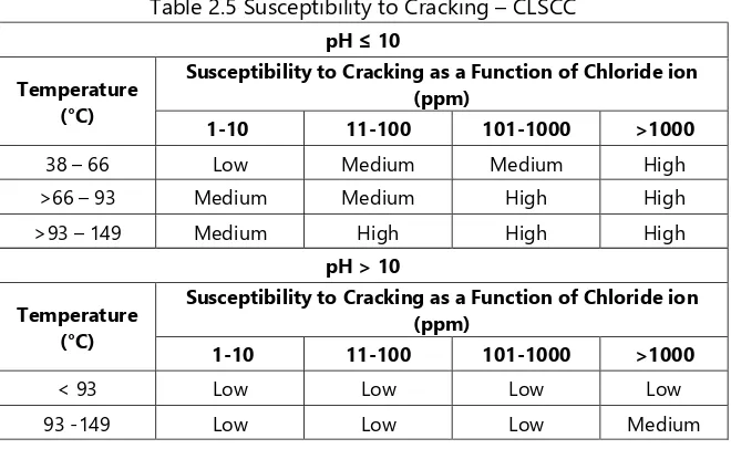
Table 2.5 Susceptibility to Cracking – CLSCC

pH ≤ 10

Temperature (°C)

Susceptibility to Cracking as a Function of Chloride ion (ppm)

1-10 11-100 101-1000 >1000

< 93 Low Low Low Low

93 -149 Low Low Low Medium

d) Based on the susceptibility in step 2.2.1.2.6.c, and determine the severity index, 𝑆_𝑉𝐼 from table 2.6.

Table 2.6 Determination of Severity Index – CLSCC

Susceptibility Severity Index –SVI

High 5000 effectiveness determined in step 2.2.1.2.6.a, and the severity index,

𝑆𝑉𝐼, from step 2.2.1.2.6.d.

Table 2.7 SCC Damage Factors – All SCC Mechanisms

SVI

Inspection Effectiveness

E 1 Inspection 2 Inspections 3 Inspections

(48)

f) Calculate the escalation in the damage factor based on the time in-service since the last inspection using the age from STEP 2 and equation (2.14). In this equation, it is assumed that the probability for cracking will increase with time since the last inspection as a result of increased exposure to upset conditions and other non-normal conditions.

𝐷𝑓𝐶𝐿𝑆𝐶𝐶 = 𝐷𝑓𝐵𝐶𝐿𝑆𝐶𝐶 (age)1.1 2.14

2.2.1.3. Consequences of Failure

The consequences of failure are the result if the asset getting failure. According to API RBI, consequences of failure assessment is performed to determining a ranking of equipment items on the basis of risk. There are four consequence categories such as; flammable, toxic consequences, non-flammable and non-toxic release and financial consequence. API RBI also provide two level consequences of failure methodology.

2.2.1.3.1. Consequence Categories

The major consequence categories are analyzed using different technique.

a) Flammable and explosive consequences are calculated using event trees to determine the probabilities of various outcomes (e.g., pool fires, flash fires, vapor cloud explosions), combined with computer modeling to determine the magnitude of the consequence. Consequence areas can be determined based on serious personnel injuries and component damage from thermal radiation and explosions. Financial losses are also determined based on the area affected by the release.

b) Toxic consequences are calculated using computer modeling to determine the magnitude of the consequence area as a result of overexposure of personnel to toxic concentrations within a vapor cloud. Where fluids are flammable and toxic, the toxic event probability assumes that if the release is ignited, the toxic consequence is negligible (i.e. toxics are consumed in the fire). Financial losses are also determined based on the area affected by the release.

(49)

21

chemical splashes and high temperature steam burns are determined based on serious injuries to personnel. Physical explosions and BLEVEs can also cause serious personnel injuries and component damage.

d) Financial Consequences includes losses due to business interruption and costs associated with environmental releases. Business interruption consequences are estimated as a function of the flammable and non-flammable consequence area results. Environmental consequences are determined directly from the mass available for release or from the release rate.

2.2.1.3.2. Methodology of Consequence Analysis 2.2.1.3.2.1. Level 1 Consequence Analysis

The Level 1 consequence analysis can be used for a limited number of representative fluids. This simplified method contains table lookups and graphs that can readily be used to calculate the consequence of releases without the need of specialized consequence modeling software or techniques.

The following simplifying assumptions are made in the Level 1 consequence analysis:

a) The fluid phase upon release can only be either a liquid or a gas, depending on the storage phase and the phase expected to occur upon release to the atmosphere, in general, no consideration is given to the cooling effects of flashing liquid, rainout, jet liquid entrainment or two-phase.

b) Fluid properties for representative fluids containing mixtures are based on average values (e.g. MW, NBP, density, specific heats, AIT)

c) Probabilities of ignition, as well as the probabilities of other release events (VCE, pool fire, jet fire, etc.) have been pre-determined for each of the representative fluids as a function of temperature, fluid AIT and release type. These probabilities are constants, totally independent of the release rate.

(50)

the impact of detection and isolation systems on release magnitude, determine the release rate and mass for consequence analysis, determine flammable and explosive consequences.

2.2.1.3.2.1.1. Calculation Procedures of Determining the Representative

Fluid and Associated Properties The calculation procedures are:

a) Select a representative fluid group from table (2.8).

Table 2.8 List of Representative Fluids Available for Level 1 Analysis

Representative

Fluid Fluid TYPE Examples of Applicable Materials

C₁-C₂ TYPE 0 methane, ethane, ethylene, LNG, fuel gas

C₃-C₄ TYPE 0 propane, butane, isobutane, LPG

C₅ TYPE 0 Pentane

C₆-C₈ TYPE 0 gasoline, naptha, light stright run, heptane

C₉-C₁₂ TYPE 0 diesel, kerosene

C₁₃-C₁₆ TYPE 0 jet fuel, kerosene, atmospheric gas oil

C₁₇-C₂₅ TYPE 0 gas oil, typical crude

C₂₅₊ TYPE 0 residuum, heavy crude, lube oil, seal oil

H₂ TYPE 0 hydrogen only

H₂S TYPE 0 hydrogen sulfide only

HF TYPE 0 hydrogen fluoride

Water TYPE 0 Water

Steam TYPE 0 Steam

acid (low) TYPE 0 acid, caustic

Aromatics TYPE 1 benzene, toluene, xylene, cumene

AICl3 TYPE 0 aluminum chloride

Pyrophoric TYPE 0 pyrophoric materials

Ammonia TYPE 0 Ammonia

Chlorine TYPE 0 Chlorine

CO TYPE 1 carbon monoxide

DEE TYPE 1 (see

note 2) diethyl ether

HCL TYPE 0 (see

note 1) hydrogen chloride

nitric acid TYPE 0 (see

note 1) nitric acid

NO₂ TYPE 0 (see _{note 1)} nitrogen dioxide

Phosgene TYPE 0 Phosgene

TDI TYPE 0 (see

note 1) toluene diisocyanate

(51)

23

Table 2.8 List of Representative Fluids Available for Level 1 Analysis (Continue)

PO TYPE 1 propylene oxide

Styrene TYPE 1 Styrene

EEA TYPE 1 ethylene glycol monoethyl ether acetate

EE TYPE 1 ethylene glycol monoethyl ether

EG TYPE 1 ethylene glycol

EO TYPE 1 ethylene oxide

Notes:

1. HCL, Nitric Acid, NO₂, and TDI are TYPE 1 toxic fluids 2. DEE is a TYPE 0 toxic fluid

b) Determine the stored fluid phase; Liquid or Vapor. c) Determine the stored fluid properties.

- MW – Molecular weight, kg/kg-mol [lb/lb-mol], can be estimated from table (2.9).

- k – Ideal gas specific heat ratio, can be estimated using equation (2.15) and the P C values as determined using table (2.9).

𝑘 = _𝐶𝐶𝑝

𝑝−𝑅 2.15

- AIT – Auto-ignition temperature, K [°R], can be estimated from table (2.9).

Table 2.9 Properties of the Representative Fluids Used in Level 1 Analysis

(52)

d) Determine the steady state phase of the fluid after release to the atmosphere, using table (2.10) and the phase of the fluid stored in the equipment as determined in step 2.2.1.3.2.1.1.b.

Table 2.10 Consequence Analysis Guidelines for Determining the Phase of a Fluid

Phase of Fluid at

API RBI Determination of Final Phase for Consequence Calculation

Gas Gas model as gas

Gas Liquid model as gas

Liquid Gas

model as gas unless the fluid boiling

point at ambient conditions is greater than 80°F, then model as a liquid

Liquid Liquid model as liquid

2.2.1.3.2.1.2. Calculation Procedure of Release Hole Size Selection

The calculation procedures are:

a) Based on the component type and table (2.11), determine the release hole size diameters (dn).

b) Determine the generic failure frequency (gffn), and the total

generic failure frequency from this table or from equation (2.16).

𝑔𝑓𝑓𝑡𝑜𝑡𝑎𝑙= ∑4𝑛−1𝑔𝑓𝑓𝑛 2.16

Table 2.11 Release Hole Sizes and Area used

Release Hole Number

Release Hole Size Range of Hole

Diameters (mm)

2.2.1.3.2.1.3. Calculation Procedure of Release Rate Calculation

The calculation procedures are:

a) Select the appropriate release rate equation as described above using the stored fluid phase

b) For each release hole size, compute the release hole size area (An) using Equation (2.17) based on dn.

𝐴𝑛= 𝜋𝑑𝑛

2

(53)

25

c) For each release hole size, calculate the release rate (Wn) with

equation 2.18 for each release area (An)

𝑊𝑛 = 𝐶_𝐶𝑑₂ x 𝐴𝑛 x 𝑃𝑠 x √(𝑘𝑥_𝑅𝑀𝑊_𝑥_𝑇𝑥_𝑠𝑔𝑐) 𝑥 (_𝑘+12 )

𝑘 𝑘−1

2.18

2.2.1.3.2.1.4. Calculation Procedure of Estimate the Fluid Inventory

Available for Release (Available Mass) The Calculation procedures are:

a) Group components and equipment items into inventory groups (table 2.12)

b) Calculate the fluid mass (masscomp) in the component being

evaluated.

c) Calculate the fluid mass in each of the other components that are included in the inventory group (masscomp,i).

d) Calculate the fluid mass in the inventory group (massinv) using

Equation (2.19)

𝑚𝑎𝑠𝑠𝑖𝑛𝑣= ∑𝑁𝑖=1𝑚𝑎𝑠𝑠𝑐𝑜𝑚𝑝,𝑖 2.19

Table 2.12 Assumption When Calculating Liquid Inventories Within Equipment

Equipment Description

Component

Type Examples

Default Liquid Volume Percent

Process Columns two or three items)

- top half - middle section - bottom half

These default values are typical of trayed distillation columns and consider liquid holdup at the bottom of the

vessel as well as the presence of chimney trays

in the upper sections

Accumulators and Drums

DRUM

OH Accumulators, Feed Drums, HP/LP Separators, Nitrogen

Storage drums, Steam Condensate

Drums

50% liquid

Typically, 2-phase drums are liquid level controlled at

(54)

Table 2.12 Assumption When Calculating Liquid Inventories Within

Default Liquid Volume Percent

Knock-out Pots and Dryers

KODRUM

Compressor Knock-outs, Fuel Gas KO Drums, Flare Drums,

Air Dryers.

10% liquid Much less liquid inventory

expected in knock-out drums

Heat Exchangers HEXSS

HEXTS

Shell and Tube Heat Exchangers

50% shell-side, 25% tube-side

Fin Fan Air Coolers FINFAN

Total Condensers, Partial Condensers, Vapor Coolers and

Liquid Coolers

25% liquid

Filters FILTER 100% full

Piping PIPE-xx 100% full, calculated for

Level 2 Analysis

e) Calculate the flow rate from a 203 mm [8 in] diameter hole (Wmax8) using equations (2.18), as applicable, with 8 32,450 n A

= A = mm2 [50.3 in2]. This is the maximum flow rate that can be added to the equipment fluid mass from the surrounding equipment in the inventory group.

f) For each release hole size, calculate the added fluid mass (massadd,n) resulting from three minutes of flow from the

inventory group using equation (2.20) where Wn is the leakage

rate for the release hole size being evaluated and Wmax8 is from

last step.

massadd,n = 180 . min [Wn , Wmax8] 2.20

g) For each release hole size, calculate the available mass for release using Equation (2.21)

(55)

27

2.2.1.3.2.1.5. Calculation Procedure of Determining the Release Type

(Continuous or Instantaneous) The Calculation procedures are:

a) For each release hole size, calculate the time required to release 4,536 kgs [10,000 lbs] of fluid.

𝑡𝑛=_𝑊𝐶3_𝑛 2.22

b) For each release hole size, determine if the release type is instantaneous or continuous using the following criteria. - If the release hole size is 6.35 mm [0.25 inches] or less, then

the release type is continuous.

- If 180 tn ≤ sec or the release mass is greater than 4,536 kgs

[10,000 lbs], then the release is instantaneous; otherwise, the release is continuous.

2.2.1.3.2.1.6. Estimate the Impact of Detection and Isolation Systems on Release Magnitude

The Calculation procedures are:

a) Determine the detection and isolation systems present in the unit.

b) Using table (2.13),select the appropriate classification (A, B, C) for the detection system.

Table 2.13 Detection and Isolation System Rating Guide

Type of Detection System Detection

Classification

Instrumentation designed specifically to detect material losses by changes in operating conditions (i.e., loss of pressure or flow) in the system

A

Suitably located detectors to determine when the material is

present outside the pressure-containing envelope B

Visual detection, cameras, or detectors with marginal coverage C

Type of Isolation System Isolation

Classification

Isolation or shutdown systems activated directly from process

instrumentation or detectors, with no operator intervention A

Isolation or shutdown systems activated by operators in the

control room or other suitable locations remote from the leak B

(56)

c) Using table (2.13), select the appropriate classification (A, B, C) for the isolation system.

d) Using (2.14) and the classifications determined in step 2.2.1.3.2.1.6.b & 2.2.1.3.2.1.6.c, determine the release reduction factor, factdi.

Table 2.14 Adjustments to Release Based on Detection and Isolation Systems

System

Classifications _{Release Magnitude Adjustment}

Reduction Factor,

factdi

Detection Isolation

A A _{Reduce release rate or mass by 25%} _0.25 durations for each of the selected release hole sizes, ldmax,n.

Table 2.15 Leak Durations Based on Detection and Isolation Systems

Detecting System Rating

Isolation System

Rating Maximum Leak Duration, ldmax

A A

20 minutes for 6.4 mm leaks 10 minutes for 25 mm leaks 5 minutes for 102 mm leaks

A B

A C

B A or B

B C

1 hour for 6.4 mm leaks 30 minutes for 25 mm leaks 20 minutes for 102 mm leaks

C A, B or C

(57)

29

2.2.1.3.2.1.7. Determining the Release Rate and Mass for Consequence

Analysis

The Calculation Procedure are:

a) For each release hole size, calculate the adjusted release rate (raten) using Equation 4.12 where the theoretical release rate

(Wn) is from step 4.4.3.b. Note that the release reduction factor

(factdi) determined in step 4.4.6.d accounts for any detection

and isolation systems that are present.

raten = Wn(1-factdi) 2.23

b) For each release hole size, calculate the leak duration (ldn) of

the release using Equation 4.13, based on the available mass (massavail,n), and the adjusted release rate (raten) Note that the

leak duration cannot exceed the maximum duration (Idmax,n)

determined in step 2.2.1.3.2.1.6.e.

𝑙𝑑𝑛= 𝑚𝑖𝑛 [{𝑚𝑎𝑠𝑠_{𝑟𝑎𝑡𝑒}𝑎𝑣𝑎𝑖𝑙,𝑛_𝑛 } , {60𝑥𝐼𝑑𝑚𝑎𝑥,𝑛}] 2.24

c) For each release hole size, calculate the release mass (massn) ,

using equation (4.14) based on the release rate (raten) from

step 2.2.1.3.2.1.3.b, the leak duration (ldn) , from step

2.2.1.3.2.1.7.b, and the available mass (massavail,n) from step

2.2.1.3.2.1.4.f.

massn = min [{raten . ldn} , massavail,n] 2.25

2.2.1.3.2.1.8. Flammable and Explosive Consequence

The Calculation Procedure are:

(58)

Table 2.16 Adjustments to Flammable Consequences for Mitigation

Inventory blowdown, coupled with isolation system classification B or higher

Reduce consequence area by 25%

0.25

Fire water deluge system and monitors

0.20

Fire water monitors only

0.05

Foam spray system

0.15

b) For each release hole size, calculate the energy efficiency correction factor, eneffn, using equation (2.26).

𝑒𝑛𝑒𝑓𝑓𝑛= 4𝑥𝑙𝑜𝑔10[𝐶4𝑥𝑚𝑎𝑠𝑠𝑛]– 15 2.26

c) Determine the fluid type, either TYPE 0 or TYPE 1 from table (2.8).

d) For each release hole size, compute the component damage consequence areas for Autoignition Not Likely, Continuous Release (AINL-CONT) (_𝐶𝐴_{𝑐𝑚𝑑,𝑛}𝐴𝐼𝑁𝐿−𝐶𝑂𝑁𝑇)_.

1) Determine the appropriate constants a (𝑎_𝑐𝑚𝑑𝐴𝐼𝐿−𝐶𝑂𝑁𝑇) and b (𝑏_𝑐𝑚𝑑𝐴𝐼𝐿−𝐶𝑂𝑁𝑇) from the table (2.17) The release phase as determined in step 2.2.1.3.2.1.1.d. will be needed to assure selection of the correct constants.

2) If the release is a gas or vapor and the fluid type is TYPE 0, then use Equation (2.27) for the consequence area and Equation (2.28) for the release rate.

𝐶𝐴𝑐𝑚𝑑,𝑛𝐴𝐼𝑁𝐿−𝐶𝑂𝑁𝑇= 𝑎(𝑟𝑎𝑡𝑒𝑛)𝑏 x (1 − 𝑓𝑎𝑐𝑡𝑚𝑖𝑡) 2.27

(59)

31

Table 2.17 Component Damage Flammable Consequence Equation Constants

Fluid

Continuous Releases Constants

Auto-Ignition Not Likely Auto-Ignition Likely

(CAINL) (CAIL)

Instantaneous Releases Constants

Auto-Ignition Not Likely Auto-Ignition Likely

(IAINL) (IAIL)

e) For each release hole size, compute the component damage consequence areas for Autoignition Likely, Continuous Release (AIL-CONT), (𝐶𝐴_{𝑐𝑚𝑑,𝑛}𝐴𝐼𝐿−𝐶𝑂𝑁𝑇)

1) Determine the appropriate constants, a (𝑎_𝑐𝑚𝑑𝐴𝐼𝐿−𝐶𝑂𝑁𝑇) and b (𝑏_𝑐𝑚𝑑𝐴𝐼𝐿−𝐶𝑂𝑁𝑇) The release phase as determined in step 2.2.1.3.2.1.1.d will be needed to assure selection of the correct constants.

(60)

𝐶𝐴_{𝑐𝑚𝑑,𝑛}𝐴𝐼𝐿−𝐶𝑂𝑁𝑇₌_{𝑎(𝑟𝑎𝑡𝑒}

𝑛)𝑏 x (1 − 𝑓𝑎𝑐𝑡𝑚𝑖𝑡) 2.29

𝑒𝑓𝑓𝑟𝑎𝑡𝑒𝑛𝐴𝐼𝐿−𝐶𝑂𝑁𝑇= 𝑟𝑎𝑡𝑒𝑛 2.30

f) For each release hole size, compute the component damage consequence areas for Autoignition Not Likely, Instantaneous Release (AINL-INST)

1) Determine the appropriate constants a (𝑎_𝑐𝑚𝑑𝐴𝐼𝑁𝐿−𝐼𝑁𝑆𝑇) and b (𝑏_𝑐𝑚𝑑𝐴𝐼𝑁𝐿−𝐼𝑁𝑆𝑇). The release phase as determined in step 2.2.1.3.2.1.1.d will be needed to assure selection of the correct constants.

2) If the release is a gas or vapor and the fluid type is TYPE 0, or the fluid type is TYPE 1, then use equation (2.31) for the consequence area and equation (2.32) for the effective release rate.

𝐶𝐴𝑐𝑚𝑑,𝑛𝐴𝐼𝑁𝐿−𝐼𝑁𝑆𝑇= 𝑎(𝑚𝑎𝑠𝑠𝑛)𝑏 x (1−𝑓𝑎𝑐𝑡_{𝑒𝑛𝑒𝑓𝑓}𝑚𝑖𝑡_𝑛 ) 2.31

𝑒𝑓𝑓𝑟𝑎𝑡𝑒𝑛𝐴𝐼𝑁𝐿−𝐼𝑁𝑆𝑇= 𝑚𝑎𝑠𝑠𝑛 2.32

g) For each release hole size, compute the component damage consequence areas for Autoignition Likely, Instantaneous Release (AIL-INST) (𝐶𝐴_{𝑐𝑚𝑑,𝑛}𝐴𝐼𝐿−𝐼𝑁𝑆𝑇)

1) Determine the appropriate constants a (𝑎_𝑐𝑚𝑑𝐴𝐼𝐿−𝐼𝑁𝑆𝑇) and b (𝑏_𝑐𝑚𝑑𝐴𝐼𝐿−𝐼𝑁𝑆𝑇). The release phase as determined in step 2.2.1.3.2.1.1.d will be needed to assure selection of the correct constants.

2) If the release type is gas or vapor, Type 0 or Type 1, then use Equation (2.31) to compute the consequence area and Equation (2.32) to compute the effective release rate.

𝐶𝐴_{𝑐𝑚𝑑,𝑛}𝐴𝐼𝐿−𝐼𝑁𝑆𝑇₌_{𝑎(𝑚𝑎𝑠𝑠}

𝑛)𝑏 x (1−𝑓𝑎𝑐𝑡_{𝑒𝑛𝑒𝑓𝑓}𝑚𝑖𝑡_𝑛 ) 2.33

(61)

33

h) For each release hole size, compute the personnel injury consequence areas for Auto-ignition Not Likely, Continuous Release (AINL-CONT) (𝐶𝐴_{𝑖𝑛𝑗,𝑛}𝐴𝐼𝑁𝐿−𝐶𝑂𝑁𝑇)

1) Determine the appropriate constants a (𝑎_𝑖𝑛𝑗𝐴𝐼𝑁𝐿−𝐶𝑂𝑁𝑇) and b (𝑏𝑖𝑛𝑗𝐴𝐼𝑁𝐿−𝐶𝑂𝑁𝑇). The release phase as determined in step

2.2.1.3.2.1.1.d will be needed to assure selection of the correct constants.

2) Compute the consequence area using Equation (2.35) where

𝑒𝑓𝑓𝑟𝑎𝑡𝑒𝑛𝐴𝐼𝑁𝐿−𝐶𝑂𝑁𝑇 is from step 2.2.1.3.2.1.8.d.

𝐶𝐴_{𝑖𝑛𝑗,𝑛}𝐴𝐼𝑁𝐿−𝐶𝑂𝑁𝑇₌_{𝑎(𝑒𝑓𝑓𝑟𝑎𝑡𝑒}

𝑛𝐴𝐼𝑁𝐿−𝐶𝑂𝑁𝑇)𝑏 x (1 − 𝑓𝑎𝑐𝑡𝑚𝑖𝑡) 2.35

i) For each release hole size, compute the personnel injury consequence areas for Auto-ignition Likely, Continuous Release (AIL-CONT) (𝐶𝐴_{𝑖𝑛𝑗,𝑛}𝐴𝐼𝐿−𝐶𝑂𝑁𝑇)

1) Determine the appropriate constants a (𝑎_𝑖𝑛𝑗𝐴𝐼𝐿−𝐶𝑂𝑁𝑇) and b (𝑏_𝑖𝑛𝑗𝐴𝐼𝐿−𝐶𝑂𝑁𝑇₎_{. The release phase as determined in step}

2.2.1.3.2.1.1.d will be needed to assure selection of the correct constants.

2) Compute the consequence area using Equation (2.36) where

𝑒𝑓𝑓𝑟𝑎𝑡𝑒𝑛𝐴𝐼𝐿−𝐶𝑂𝑁𝑇 is from step 2.2.1.3.2.1.8.e.

𝐶𝐴𝑖𝑛𝑗,𝑛𝐴𝐼𝐿−𝐶𝑂𝑁𝑇= 𝑎(𝑒𝑓𝑓𝑟𝑎𝑡𝑒𝑛𝐴𝐼𝐿−𝐶𝑂𝑁𝑇)𝑏 x (1 − 𝑓𝑎𝑐𝑡𝑚𝑖𝑡) 2.36

j) For each release hole size, compute the personnel injury consequence areas for Auto-ignition Not Likely, Instantaneous Release (AINL-INST) (𝐶𝐴_{𝑖𝑛𝑗,𝑛}𝐴𝐼𝑁𝐿−𝐼𝑁𝑆𝑇)

1) Determine the appropriate constants a (𝑎_𝑖𝑛𝑗𝐴𝐼𝑁𝐿−𝐼𝑁𝑆𝑇) and b (𝑏_𝑖𝑛𝑗𝐴𝐼𝑁𝐿−𝐼𝑁𝑆𝑇). The release phase as determined in step 2.2.1.3.2.1.1.d will be needed to assure selection of the correct constants.

2) Compute the consequence area using equation (2.36) where

𝑒𝑓𝑓𝑟𝑎𝑡𝑒𝑛𝐴𝐼𝑁𝐿−𝐼𝑁𝑆𝑇is from step 2.2.1.3.2.1.1.f.