POPULATION DYNAMICS WITH SYMMETRIC AND
ASYMMETRIC HARVESTING
Jaffar Ali1, David Perry2, Sarath Sasi3, Jessica Schaefer4 Brian Schilling3, R. Shivaji3 and Matthew Williams5
1 Department of Mathematics, Florida Gulf Coast University e-mail: [email protected]
2 Department of Mathematics, New York University e-mail: [email protected]
3 Department of Mathematics, Center for Computational Sciences Mississippi State University, Mississippi State, MS 39762-9715 USA e-mail: [email protected], [email protected], [email protected]
4 Department of Mathematics, Northern Arizona University e-mail: [email protected]
5 Department of Mathematics, Clarkson State University e-mail: [email protected]
Honoring the Career of John Graef on the Occasion of His Sixty-Seventh Birthday Abstract
We study the positive solutions to steady state reaction diffusion equations with Dirichlet boundary conditions of the forms:
−u′′=
λ[au−bu2−c], x∈(L,1−L),
λ[au−bu2], x∈(0, L)∪(1−L,1), (A) u(0) = 0 =u(1),
and
−u′′=
λ[au−bu2−c], x∈(0,12),
λ[au−bu2], x∈(12,1), (B) u(0) = 0 =u(1).
Hereλ, a, b, candLare positive constants with 0< L < 12. Such steady state equations arise in population dynamics with logistic type growth and constant yield harvesting. Here u is the population density, 1λ is the diffusion coefficient andcis the harvesting effort. In particular, model A corresponds to a symmetric harvesting case and model B to an asymmetric harvesting case. Our objective is to study the existence of positive solutions and also discuss the effects of harvesting. We will develop appropriate quadrature methods via which we will establish our results.
Key words and phrases: Population dynamics, reaction diffusion, harvesting, sym-metric, asymmetric.
1
Introduction
In [9] the authors study the nonlinear boundary value problem
(
−∆u=au−bu2−ch(x), x∈Ω,
u= 0, x∈∂Ω, (1)
arising in population dynamics. Here Ω is a smooth bounded region with ∂Ω ∈ C2,
u is the population density, au −bu2 represents logistic growth where a > 0, b > 0 are constants. Here h is assumed to be a smooth function representing the intrinsic properties of the region while c≥0 represents the harvesting effort. The assumptions in the development of this steady state model are: (i) the species disperses randomly in the bounded environment; (ii) the reproduction of the species follows logistic growth; (iii) the boundary is hostile to the species; and (iv) the environment is homogeneous (i.e., the diffusion coefficient is independent of spatial variable x).
Here we extend this study to cases where h(x) is a non-smooth function. However we restrict our analysis to the one-dimensional case with Ω = (0,1) and study the following two models:
Model A
−u′′=
λ[au−bu2−c], x∈(L,1−L),
λ[au−bu2], x∈(0, L)∪(1−L,1), (A)
u(0) = 0 =u(1);
Model B
−u′′=
λ[au−bu2−c]; x∈(0,1
2)
λ[au−bu2]; x∈(1
2,1)
(B)
u(0) = 0 =u(1).
There has been a raging controversy over the decline of western Atlantic bluefin tuna since the 1970s (see [8]). The U.S. fishing industries demand that the bluefin tuna movements between the western and eastern Atlantic be considered for a better assessments of the effect of ‘overfishing’ of bluefin by fishermen in central and eastern Atlantic, including the Mediterranean Sea. The model B is a simplified representation of the bluefin tuna population in the Atlantic Ocean in which we focus on the diffusion effects (the convection effects are not considered). It tries to capture the scenario where fishing is restricted to one half of the ocean. The relevance of the study is to see if such regulations can improve the depleting stock of fish in the Atlantic (see also [3] and [10]).
We analyze these problems by modifying the quadrature method discussed in [6] to accommodate such models with discontinuous reaction terms. For further information on the quadrature method see [2] and [4].
In Section 2 the quadrature method that was developed in [6] is briefly outlined. In Section 3 and Section 4 we extend the quadrature method for model A and model B respectively, and study the existence of a positive solution. Though in both models (A) and (B), in one of the harvesting regions the harvesting effort is zero, our methods easily extend to models with unequal harvesting rates in different regions. In Section 5, we provide various computational results on the bifurcation diagrams of positive solutions.
2
Preliminaries
Here we describe the quadrature method that has been used to prove our results. Consider the boundary value problem
(
−u′′ =λf(u), x∈(0,1),
u(0) = 0 =u(1), (2)
wheref : [0,∞)→(0,∞) is aC1 function andλ is a positive parameter. Supposeuis a solution of (2) in (0,1) such thatu′(x
0) = 0 forx0 ∈ (0,1). Thenu(x0+x) =u(x0−x) for all x∈[0, c) where c= min{x0,1−x0}. This follows by noting the fact that both
v(x) :=u(x0+x) and w(x) :=u(x0−x) satisfy the initial value problem
−z′′(x) =λf(z(x)),
z(0) =u(x0),
z′(0) = 0.
Hence if u is a positive solution of (2) then u must be symmetric about x = 1 2, increasing on (0,12) and decreasing on (12,1). Letρ =||u||∞(note thatu(12) = ρ). Now multiplying (2) by u′(x) we obtain
−u
′(x)2 2
′
=λ(F(u(x)))′ (3)
where F(s) :=Rs
0 f(t)dt, and integrating from 0 to 1
2 we get
u′(x) =p2λ[F(ρ)−F(u(x))] 0< x < 1
2. (4)
Here we have used u(12) =ρ;u′(1
2) = 0. We rewrite (4) as
u′(x)
p
[F(ρ)−F(u(x))] =
√
and integrate fromu(0) = 0 tou(x) after making the substitution z =u(x). This gives
Z u(x)
0
dz
p
[F(ρ)−F(z)] =
√
2λx 0< x < 1
2. (6)
Further since u(1
2) =ρ we obtain
√
λ=√2
Z ρ
0
dz
p
[F(ρ)−F(z)] :=G(ρ). (7)
Thus, if there exists a positive solution u of (2) with u(1
2) = ρ, then ρ must be such that G(ρ) exists and satisfy √λ = G(ρ). Since f(ρ) > 0 and F(ρ) > F(z) for all 0≤z ≤ρ, it follows thatG(ρ) exists for allρ >0. (AlsoG(ρ) is a continuous function with G(0) = 0.)
Now suppose there exists ρ > 0 such that √λ = G(ρ). Define u(x) for x ∈ [0,12] using (6). It can be shown that u is a C2 function that satisfies (2). Thus (2) has a positive solution u with u(12) = ρ > 0 iff √λ = G(ρ). Hence by analyzing G(ρ) for ρ ∈ (0,∞) we can precisely discuss the existence, non-existence and multiplicity of positive solutions as λ varies. Further, when the solution exists, (6) defines the solution.
3
Symmetric Constant Yield Harvesting
In this section we consider the model A with harvesting allowed only in the interior. Quadrature methods are developed for the regions with and without harvesting sep-arately to prove the existence of a positive solution. We call such classes of positive symmetric solutions as ‘Type I’ solutions. In this section we consider Type I solutions. Let f(u) :=au−bu2 and ˜f(u) :=au−bu2−c.
1 0.5
L 1-L
x
Ρ
Σ
uHxL
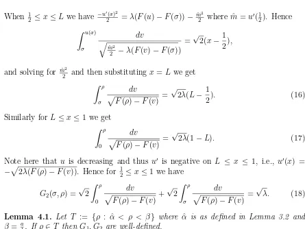
We first consider the interval (L,12). On the interval (L,12) we have
−u′′ =λf˜(u).
Using similar calculations as in Section 2, we have
u′ =
2), solutions of the model A will satisfy
As proceeding in the previous case we observe that the solutionu of model A on (0, L) satisfies
In order for u to be a C1 solution of model A, it is necessary that
u′(L+) =u′(L−).
Hence
m2
2 =λ[ ˜F(ρ)−F˜(σ) +F(σ)]. Substituting in (12) and simplifying we get
Lemma 3.1. Let S := {ρ : ˆα < ρ < βˆ} where αˆ = 43ba−
q
3a2
−16bc
3
and βˆ = a+√a2
−4bc
2b . If ρ∈S then G1, G2 are well-defined.
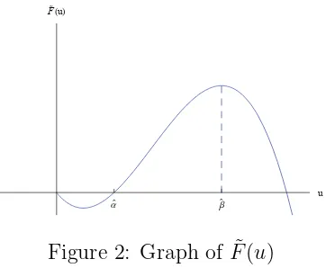
Proof. We note here that ˆα is the first non-zero root of ˜F(u) = au22 − bu33 −cuand ˆβ
is the first largest positive root of ˜F′(u) = ˜f(u).
Α` Β`
u FHuL
Figure 2: Graph of ˜F(u)
It is clear from the graph of ˜F that ˜F(ρ)−F˜(v) is positive for allv ∈(0, ρ) only if
ρ ∈( ˆα,βˆ). Further, for ρ ∈S, ˜f(ρ)>0. Hence G1 is well-defined for ρ ∈S. Now we observe that for v ≤σ,
F(ρ)−F(v)−c(ρ−σ)≥F(ρ)−F(v)−c(ρ−v) = ˜F(ρ)−F˜(v).
Hence G2(σ, ρ) is also well-defined for all ρ∈S.
Remark 3.1. Note that S is non-empty iff c≤ 316a2b.
Lemma 3.2. Letρ∈S be fixed, then there exists a uniqueσ∗(ρ)such thatG
1(σ∗(ρ), ρ) =
G2(σ∗(ρ), ρ). Moreover, if u is a positive solution of (A) then u(L) =σ∗(ρ).
Proof. We observe from (10) that G1 is non-negative, decreasing and G1(ρ, ρ) = 0. Similarly from (13), we have G2 is non-negative, increasing and G2(0, ρ) = 0. We also have that G1(0, ρ) > 0 and G2(ρ, ρ) > 0. Thus G1 −G2 a continuous function with (G1−G2)(0, ρ) >0 and (G1−G2)(ρ, ρ) < 0. Hence by Intermediate Value Theorem there exists a σ∗(ρ) such that (G
1−G2)(σ∗(ρ), ρ) = 0. i.e. G1(σ∗(ρ), ρ) =G2(σ∗(ρ), ρ). As G1−G2 is strictly decreasing such a σ∗(ρ) is unique.
Clearly, if u is a positive solution of (A) satisfying (10) and (13), then u(L) =
σ∗(ρ).
Theorem 3.1. Letρ∈S, λ >0and letr1 andr2 be the zeros off˜(u). (A) has a posi-tive solution iff√λ∈Range(H), where H(ρ) =G2(σ∗(ρ), ρ)[orH(ρ) =G1(σ∗(ρ), ρ)]. Moreover, if ρ = r1 (or ρ = r2) and satisfies F(r1) = m
2
2λ (or F(r2) = m2
2λ) then
Proof. Letube a positive solution of (A). By Lemma 3.2√λ ∈Range(H). Conversely
let √λ∈Range(H). Let u(x) be symmetric atx= 12 and be defined as
u(x) =
(
u1(x), x∈(0, L),
u2(x), x∈(L,12],
(14)
where u1, u2 satisfies (11) and (8), respectively. Since
√
λ ∈ Range(H), there exists
ρ ∈ S such that √λ = H(ρ), that is G2(σ∗(ρ)) =
√
λ = G1(σ∗(ρ)), thus u clearly satisfies (A). Hence uis positive solution of (A).
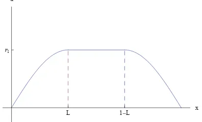
L 1-L
x r1
u
Figure 3: Typical Type I solution when ρ=r1
We note that ˜f(r1) = 0 and thus u′′(L) = 0. Also since F(r1) = m
2
2λ, we have
u′(L−) = 0, and by continuity onu′,u′(L) = 0. It is easy to see thatu ≡r
1 on (L,1−L) sinceu(L)−r1 = 0 =u(1−L)−r1, (u(L)−r1)′ =u′(L) = 0 =u′(1−L) = (u(1−L)−r1)′ and (u(L)−r1)′′=u′′(L) = 0 =u′′(1−L) = (u(1−L)−r1)′′. Hence the claim.
4
Asymmetric Harvesting
In this section we analyze existence of solutions to model B using the quadrature method. We call such classes of positive asymmetric solutions as ‘Type II’ solutions. In this section we consider Type II solutions. Let ˜f(u) := λ[au− bu2 −c], f(u) :=
λ[au−bu2] andL be the point at which uis maximum.We consider the following two cases:
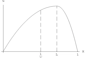
Case 1: Maximum value is achieved at a point L > 12
L
Figure 4: Typical Type II solution for case 1
L 1
Figure 5: Typical Type II solution for case 2
4.1
Case 1 :
L >
12Lemma 4.2. Letρ∈T be fixed, then there exists a uniqueσ∗(ρ)such thatG similarly as in the Lemma 3.2.
Theorem 4.1. Let ρ ∈ T, L ≥ 12 and λ > 0. (B) has a positive solution iff √λ ∈ Range(H), where H(ρ) =G2(σ∗(ρ), ρ) [or H(ρ) =G1(σ∗(ρ), ρ)].
Proof. Proof follows similarly as in the Theorem 3.1.
4.2
Case 2 :
L <
12Theorem 4.2. (B) has no positive solution of Type II with L < 12.
Therefore
Hence no positive solution exists for Case 2.
5
Computational Results
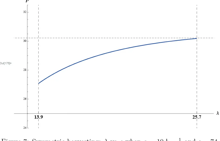
In this section we discuss the results obtained using M athematica computation of bifurcation curves of positive solutions developed in Sections 3 and 4 for models A & B. Figure 7 is the bifurcation diagram of the symmetric harvesting problem (A) with parameter values a= 10, b= 14,c= 74 and L= 13. Based on our discussion in Section
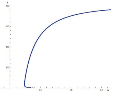
Figures 8 and 9 give the bifurcation diagram of the symmetric harvesting problem (A) with parameter values a= 100, b= 1
Out[424]=
0.2401 0.3787 Λ
20 40 60 80 100
Ρ
Figure 8: Symmetric harvesting: λ vs ρ when a= 100,b= 1
4 and c= 74
Here again the the set S is non-empty only for ρ ∈ (1.484,399.259). In Figure 8, we notice that for higher birth rates (i.e. large a such as a = 100) there exists two solutions forλ ∈(0.2401,0.3787) .
Figure 9: λ vs ρ when a= 100,b= 14 and c= 74 - (2 solutions)
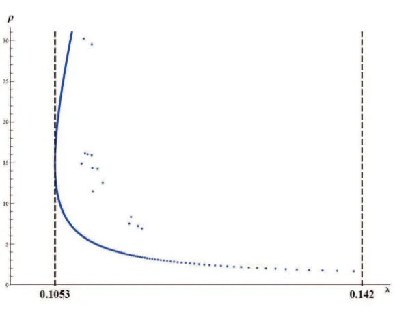
Figure 10 is the bifurcation diagram of the asymmetric harvesting problem (B) with parameter values a = 10, b = 14 and c = 74. Here ρ has to lie in the interval (26.536,40) for the setT in Theorem 4.2 to be non-empty.
Out[530]=
3.5 68.8 Λ
10 12 14 16 18 20 22 24
Ρ
Figure 10: Asymmetric harvesting: λ vs ρ when a= 10, b= 14 and c= 74
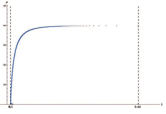
Figure 12: Asymmetric harvesting: λ vs ρ when a= 100, b = 14 and c= 74
References
[1] H. Berestycki, L. A. Caffarelli and L. Nirenberg, Inequalities for second order elliptic equations with applications to unbounded domains I. A celebration of John F. Nash, Jr.,Duke Math. J. 81 (1996), 467-494.
[2] K. J. Brown, M. M. A. Ibrahim and R. Shivaji, S-shaped bifurcation curves,Nonlin. Anal. 5 (5) (1981), 475-486.
[3] B. A. Block,et al., Migratory movements, depth preferences, and thermal biology of Atlantic bluefin tuna,Science293(2001), 1310-1314 [http://www.sciencemag.org]. [4] A. Castro and R. Shivaji, Nonnegative solutions for a class of nonpositone problems,
Proc. Roy. Soc. Edin. Sect. A 108 (1988), 291-302.
[5] A. Castro, C. Maya and R. Shivaji, Nonlinear eigenvalue problems with semiposi-tone structure, Electron. J. Diff. Eqns.5 (2000), 33-49.
[6] T. Laetsch, The number of solutions of a nonlinear two point boundary value prob-lem, Indiana Univ. Math. J.20 (1) (1970), 1-13.
[7] P. L. Lions, On the existence of positive solutions of semiliniear elliptic equations, Siam Rev. 24 (1982), 441-467.
[9] S. Oruganti, J. Shi and R. Shivaji, Diffusive equations with constant yield harvest-ing, I: steady states, Trans. Amer. Math. Soc.354 (2002), 3601-3619.