Quasi-Exactly Solvable Schr¨
odinger Operators
in Three Dimensions
M´elisande FORTIN BOISVERT
Department of Mathematics and Statistics, McGill University, Montr´eal, Canada, H3A 2K6 E-mail: [email protected]
URL: http://www.math.mcgill.ca/boisvert/
Received October 01, 2007, in final form November 02, 2007; Published online November 21, 2007 Original article is available athttp://www.emis.de/journals/SIGMA/2007/109/
Abstract. The main contribution of our paper is to give a partial classification of the quasi-exactly solvable Lie algebras of first order differential operators in three variables, and to show how this can be applied to the construction of new quasi-exactly solvable Schr¨odinger operators in three dimensions.
Key words: quasi-exact solvability; Schr¨odinger operators; Lie algebras of first order diffe-rential operators; three dimensional manifolds
2000 Mathematics Subject Classification: 81Q70; 22E70; 53C80
1
Introduction
Recall that a Schr¨odinger operator on a n-dimensional Riemannian manifold (M, g) is a second order linear differential operator of the form
H0 =−1
2∆ +U,
where ∆ is the Laplace–Beltrami operator andU is the potential function for the physical system under consideration. A question of fundamental interest in quantum mechanics is to construct eigenfunctions ψof the Schr¨odinger operatorH0. One approach to this problem, which is based
on the representation theory of Lie algebras, is to consider Schr¨odinger operators H0 which are
quasi-exactly solvable, in a sense that will be defined below.
We begin by considering the case of a general linear second-order differential operator H, given in local coordinates by
H= n
X
i,j=1
Aij∂i∂j+ n
X
i=1
Bi∂i+C.
The operatorHis said to beLie algebraic if it is an element of the universal enveloping algebra of g, a finite dimensional Lie algebra of first order differential operators. More explicitly,
H= m
X
a,b=1
CabTaTb+ m
X
a=1
CaTa+C0, (1)
where
Ta=va+ηa, 1≤a≤m, (2)
if one can find explicitly a finite dimensional g-module N of smooth functions, i.e., if N = {h1, . . . , hr} with Ta(N) ⊂ N for all 1 ≤ a ≤ m. A Lie algebraic operator H, is said to be quasi-exactly solvable if it lies in the universal enveloping algebra of a quasi-exactly solvable Lie algebra of first order differential operators. Obviously, H(N) ⊂ N, i.e. the moduleN will be fixed by the operator H. Moreover, if the functions contained in the module N are square integrable with respect to the Riemannian measure√gdx1· · ·dxn, wheregis the determinant of the covariant metric, the operatorHis said to be anormalizablequasi-exactly solvable operator. We can see from the above definitions that the formal eigenvalue problem for quasi-exactly solvable Schr¨odinger operators can be solved partially by elementary linear algebraic methods. Indeed, the operatorHis self-adjoint with respect to the inner product associated to the standard measure, therefore the restriction ofHto the finite dimensional moduleN is a Hermitian finite dimensional linear operator. Thus, one can in principle, computer= dim(N) eigenvalues ofH, counting multiplicities, by diagonalizing ther×r matrix representingH in a basis ofN.
It seems that the concept of a “spectrum generating algebra” was first introduced by Goshen and Lipkin in [15] in 1959. However, this paper did not seem to have been be noticed by the community and, ten years later, spectrum generating algebras were independently rediscovered by two groups of physicists, see [2] and [5]. Their work was an impetus for further research in this area as one can see by browsing in the two volume set of reprints [3] and the conference proceedings [16]. A survey of the history and the contribution papers related to the spectrum generating algebras is given in the review paper of B¨ohm and Ne’eman, which appears at the beginning of [4]. In the early 1980’s, Iachello, Levine, Alhassid, G¨ursey and collaborators ex-hibited applications of spectrum generating algebras to molecular spectroscopy; a survey of the theory and applications is given in the book [17]. In these applications, both nuclear and spec-troscopic, the relevant Hamiltonian is a Lie algebraic operator in the sense described previously. Finally, the analysis of a new class of Schr¨odinger operators, the quasi-exactly solvable class, was initiated in late 1980’s by Shifman, Turbiner and Ushveridze, see [23,24, 25]. A survey of the theory and applications of quasi-exactly solvable systems in physics is given in [26].
There exists a complete classification of quasi-exactly solvable Schr¨odinger operators in one dimension. In two dimensions, this classification is in principle complete. Indeed, all the Lie al-gebraic linear differential operators for which the formal spectral problem is solvable are known. The question of determining if the operator is equivalent to a Schr¨odinger operator will be discussed below. The main contribution of our paper is to extend these results to three dimen-sions by giving a partial classification of the quasi-exactly solvable Lie algebras of first order differential operator in three variables, and showing how this can be applied to the construction of new quasi-exactly solvable Schr¨odinger operators in three dimensions. Our work is based on the classification of finite dimensional Lie algebras of vector fields in three dimensions begun by Lie in [18] and completed by Amaldi in [1].
Let g(ij) be the contravariant metric of the manifold M in a local coordinate chart, eg its
determinant and g the determinant of the covariant metric. In that setting, a Schr¨odinger operator reads locally as
H0 =−
1 2
n
X
i,j=1
gij∂ij +∂i(gij)∂j−
gij∂i(eg) 2eg ∂j
+U.
Recall that a quasi-exactly solvable second order operator is not, in general, a Schr¨odinger operator. However this operator might be equivalent to a Schr¨odinger operator in a way that preserves the formal spectral properties of the operators under consideration. The appropriate notion of equivalence, which will be used throughout our work, is the following. Two differential operators are locally equivalent if there is a gauge transformation H → µHµ−1, with gauge
verify if a general second order differential operator H is equivalent to a Schr¨odinger operator with respect to this notion of equivalence. Indeed, every second order linear differential operator can be given locally by
H=−1 2
n
X
i,j=1
gij∂ij+ n
X
i
hi∂i+U.
If the contravariant tensorg(ij) is non-degenerate, that is ifg does not vanish, the operator can
be expressed as
H=−1
2∆ +V~ +U, (3)
where V~ = bi∂i is a vector field. For this operator to be locally equivalent to a Schr¨odinger operator, the vector field V~ has to be a gradient vector field with respect to the metric g(ij).
Locally, this will be the case if and only ifω =gijbjdxi, the one form associated toV~, is closed. For this reason, this condition is named theclosure condition. Note that ifV~ =∇(λ), the gauge factor is given by eλ2.
Given an operator of the form (1), the closure conditions can be easily verified provided the contravariant metricg(ij)is non-degenerate. Indeed, these conditions can be written as algebraic constraints on the coefficients Cab and Cc, and are the Frobenius compatibility conditions for an overdetermined system that will be described later.
An important point to keep in mind is that the class of quasi-exactly solvable operators is invariant under local equivalence. Indeed, suppose His a quasi-exactly solvable operator which is gauge equivalent to an other operator H0 under the rescaling µ. If H lies in the universal
enveloping algebra of g, whose g-module is N, one can easily show that H0 is quasi-exactly
solvable with respect to the finite dimensional Lie algebra
e
g=µ·g·µ−1=µ·T·µ−1 |T ∈g
which is isomorphic tog and posses the finite-dimensionaleg-module
e
N =µ· N ={µ·h |h∈ N }.
Note however that the gauge factor is not necessarily unitary. Thus, a gauge transformation does not necessarily preserve the normalizability property of the functions inN. Therefore, the class of normalizable quasi-exactly solvable operators is not invariant under our local equivalence. We now give an example of a normalizable quasi-exactly solvable Schr¨odinger operator in three variables.
Example 1. In this example we consider the quasi-exactly solvable Lie algebrag∼=sl(2)×sl(2)×
sl(2). With the standard notation p = ∂x∂ , q = ∂y∂ and r = ∂z∂, this Lie algebra representation can be spanned by the following first order differential operators
T1 =p, T2 =xp, T3 =x2p−x, T4 =q, T5=yq, T6 =y2q−y, T7 =r, T8=zr, T9=z2r−z.
Then, the finite dimensional module of smooth functions
Nmxmymz :={xiyjzk|0≤i≤mx, 0≤j≤my, 0≤k≤mz}
is a g-module provided mx = my = mz = 1. With the following choice of coefficients, one constructs the quasi-exactly solvable operator
where{Ta, Tb}=Ta(Tb)+Tb(Ta). The induced contravariant metric associated to this operator is computed to be the following positive definite matrix
g(ij)=
(x2+ 1)2 0 (x2+ 1)(z2+ 1)
0 y4+ 4y2+ 1 0
(x2+ 1)(z2+ 1) 0 2(z2+ 1)2
, (4)
whose determinant is g = (x2 + 1)2(y4 + 4y2+ 1)(z2 + 1)2. Then, with respect to this non-degenerate metric, the operator Hcan also be described as
−2H= ∆ +V~ +U,
whereV~ =−2(x3+x+z+zx2)p−2(2y+y3)q−2(2z3+ 2z+x+xz2)r.It is not hard to verify, always with respect to the metric (4), that the first order termV~ is the gradient of the function λ=−ln(x2+ 1)−1/2 ln(y4+ 4y2+ 1)−ln(z2+ 1). Hence, by considering the gauge factor
µ=eλ2 = (x2+ 1)−1/2(y4+ 4y2+ 1)−1/4(z2+ 1)−1/2,
the operatorH is gauge equivalent to a Schr¨odinger operator
−2H0 = ∆ +U,
were the potential is a rational function ofy. Furthermore, it is not hard to show that, after the gauge transformation, the functions inNe111={µ·xiyjzk|0≤i, j, k≤1}are square integrable
with respect to √gdxdydz. Recall here thatg is the determinant of the covariant metric, hence √g=µ2. Thus, fori,j,keither 0 or 1, one can use Fubini’s theorem to decompose the integral
ZZZ
R3
(µxiyjzk)2µ2dxdydz=
ZZZ
R3
x2iy2jz2k
(x2+ 1)2(y4+ 4y2+ 1)(z2+ 1)2dxdydz,
into the product of three finite integrals in one variable. Consequently the operator H0 is
a normalizable quasi-exactly solvable Schr¨odinger operator and it is possible to compute eight eigenfunctions by diagonalizing the matrix obtained by restricting H to N. For this operator, one gets two eigenvalues,−3 and 1, both of multiplicity four. The eight eigenfunctions associated to these two eigenvalues are respectively,
ψ−3,1=−1 +xz, ψ−3,2=y−xyz, ψ−3,3=xy+yz, ψ−3,4 =x+z,
ψ1,1=y+xyz, ψ1,2 =−x+z, ψ1,3 =−xy+yz, ψ1,4 = 1 +xz.
Finally, one gets eight eigenfunctions of the Schr¨odinger operator H0 by scaling each of these
functions by the gauge factor µ.
In general, there is no a-priori method for testing whether a given differential operator is Lie algebraic or quasi-exactly solvable. However, one can try to perform a classification of these operators under local equivalence using the four-step general method of classification described by Gonz´alez-L´opez, Kamran and Olver in [11].
The first step toward the classification of normalizable quasi-exactly solvable Schr¨odinger operators is to classify the finite dimensional Lie algebras of first order differential operators up to diffeomorphism and rescaling. Then, the task is to determine which of these equivalence classes admit a finite dimensional g-module N of smooth functions. Then, from the quasi-exactly solvable Lie algebras found in the second step, one can construct second order differential operator as described in (1) from any choice of coefficients Cab, Cc, and C0. The third step
can be performed by verifying the closure condition. Finally, the last step in this classification problem is to check if the functions contained in theeg-moduleNe are square integrable.
As mentioned previously, the entire classification has been established in one dimension. In the scope of the first two steps, every quasi-exactly solvable Lie algebra is locally equivalent to a subalgebra of the Lie algebra
gn= Span
∂ ∂x, x
∂ ∂x, x
2 ∂
∂x−nz ,1
,
wherenis a non negative integer, see [13] for more details. Then, once a second order differential operator is constructed, since all one forms are closed in one dimension, such operator will always be equivalent to a Schr¨odinger operator, reducing the third step to a trivial step. Finally Gonz´alez-L´opez, Kamran and Olver determined in [10] necessary and sufficient conditions for the normalizability of the eigenfunctions of the quasi-exacly solvable Schr¨odinger operators.
In two dimensions, the first two steps of the classification problem were determined by the same authors in [12] and [14]. Based upon Lie’s classification of Lie algebras of vector fields, see [18], a complete classification of the quasi-exactly solvable Lie algebras g of first order differential operators, together with their finite dimensional g-modules, was completed. The case of two complex variables is discussed in the first two papers while the third paper completed the classification by considering operators on two real variables. However, the last two steps are not yet completed but a wide variety of normalizable quasi-exactly solvable Schr¨odinger operators has been exhibited, see for instance [11,13] and [14].
In the next section, a partial classification of quasi-exactly solvable Lie algebras of first order differential operators in three dimensions is given. While these two first steps were successfully completed in one and two dimensions, only part of this work is now done in three dimensions. However, these new quasi-exactly solvable Lie algebras can be used to seek new quasi-exactly solvable Schr¨odinger operators in three dimensional space. The last section of this paper is de-voted to the description of new quasi-exactly solvable Schr¨odinger operators in three dimensions. Eigenvalues are also computed for two families of Schr¨odinger operators. These eigenvalues are part of the spectrum of the operators and their eigenfunctions, together with their nodal sur-faces, are exhibited. In addition, a connection is made between the separability theorem proved in [6] and the quasi-exactly solvable Schr¨odinger operators on flat manifold. The quasi-exactly solvable models obtained in our paper are new as far as we can tell. In particular they are not part of the list of multi-dimensional quasi-exactly solvable models obtained in [26] by the method of inverse separation of variables.
2
Classif ication of quasi-exactly solvable Lie algebras
of f irst order dif ferential operators
2.1 Lie algebras of f irst order dif ferential operators
Our goal in this section is to give a partial classification of quasi-exactly solvable Lie algebras of first order differential operators in three dimensions. A first step toward this goal is to obtain a classification of the finite dimensional Lie algebras g of first order differential operators. After this is done, the next step is to impose the existence of an explicit finite dimensional g -moduleN of smooth functions. To this end, we will first summarize the basic theory underlying the classification of Lie algebras of first order differential operators.
a semidirect product of these two spaces, D1(M) = V(M)⋉F(M). Indeed, each element T inD1(M) can be written into a sum T =v+η and the Lie bracket is given by
[T1, T2] = [v1, v2] +v1(η2)−v2(η1), where Ti =vi+ηi ∈ D1(M). (5)
Note that the spaceF(M) is also aD1(M)-module with T(ζ) =v(ζ) +η·ζ. Consequently, any finite dimensional Lie algebra of first order differential operators gcan be written as
T1 =v1+η1, . . . , Ts=vs+ηs, Ts+1=ζ1, . . . , Ts+r =ζr, (6)
wherev1, . . . , vs are linearly independent vector fields spanningh⊂ V(M), as-dimensional Lie algebra and where the functionsζ1, . . . , ζr act as multiplication operators and spanM ⊂ F(M) a finite dimensional h-module. Note that restrictions need to be imposed to the functions ηi for g to be a Lie algebra. Indeed, without the cohomological conditions that will be described below, the Lie bracket given in (5) does not necessarily return an element in the Lie algebra g. For T =v+η, we define a 1-cochain F :h → F(M) by the linear map hF;vi = η. Since any function ζ ∈ M can be added to T without changing the Lie algebra g, this map is not well defined. To deal with this issue, we should therefore interpret F as a F(M)/M-valued 1-cochain. Thus, from the Lie bracket given in (5), it is straightforward to see that g is a Lie algebra if and only if the 1-cochainF satisfies the bilinear identity
vihF;vji −vjhF;vii − hF; [vi, vj]i ∈ M, vi, vj ∈h. (7)
In terms of Lie algebra cohomology, this condition can be restated as follow, hδ1F;vi, vji ∈ M
for allvi, vj inh, i.e.F is aF(M)/M-valued 1-cocycle on h. (See [7] for a detailed description of Lie algebra cohomology.)
This classification of Lie algebras of first order differential operators would not be complete without considering the local equivalences between the Lie algebras. Indeed, if a gauge trans-formation with gauge factor µ=eλ, is performed on an operator T =v+η ing, the resulting differential operator Te =eλ·T ·e−λ =v+η−v(λ) will only differ fromT by the addition of a multiplication operator v(λ). Again, this can be expressed in cohomological terms. Indeed, under the 0-coboundary map δ0 :h→ F(M)/M defined byhδ0λ;vi=v(λ), the multiplication
factor v(λ) can be interpreted as the image, or the 0-coboundary, of the function λ. Hence, combining these two observations, it is possible to conclude that the map F is an element in H1(h,F(M)/M) = kerδ1/Imδ0. Thus, if two differential operatorsg andeg are equivalent with
respect to a change of variables ϕ and a gauge transformation given by µ = eλ, these two operators will correspond to equivalent triples (h,M,[F]), and (eh,Mf,[Fe]), where eh = ϕ∗(h),
f
M=ϕ∗(M), andFe=ϕ∗◦F◦ϕ −1
∗ +δ0λ. This is summarized in the following theorem.
Theorem 1. There is a one to one correspondence between equivalence classes of finite dimen-sional Lie algebras g of first order differential operators onM and equivalence classes of triples (h,M,[F]),where
1) h is a finite dimensional Lie algebra of vector fields; 2) M is a finite dimensional h-module of functions; 3) [F]is a cohomology class in H1(h,F(M)/M).
Hence the general classification of finite dimensional Lie algebras of first order differential operators gcan be bring down to the classification of triples (h,M,[F]) under local changes of variables.
distinguishes between the imprimitive Lie algebras, for which their exists an invariant foliation of the manifold, and the primitive Lie algebras, for which no such foliation exists. Lie’s work gives a description of the eight different classes of primitive Lie algebras and, based under the possible foliations of the manifold, the imprimitive Lie algebras are subdivided into the following three types:
I. The manifold admits locally an invariant foliation by surfaces that does not decompose into a foliation by curves.
II. The manifold admits locally an invariant foliation by curves not contained in a foliation by surfaces.
III. The manifold admits locally an invariant foliation by surfaces that does decompose into a foliation by curves.
Observe that these three types are not necessarily exclusive. For instance, the Lie algebra
h={p, q, xq, xp−yq, yp, r}belongs to the first two types. The underlying manifold R3 admits
a first indecomposable foliation by planes ∆ := {z = constant} and also admits an second invariant foliation by straight lines Φ :={x= constant} ∩ {y= constant} not contained in any invariant surfaces. Lie classified the algebras of type I and II, giving respectively twelve and twenty-one different classes of Lie algebras. Few years latter, the 103 classes of Lie algebras of the third type were exhibited by Amaldi.
The number of finite dimensional Lie algebras of vector fieldshis large and it did not seem reasonable to consider all the 154 classes. For this first classification attempt, we have chosen to focus on the algebras which seem promising in our aim to construct new quasi-exactly solvable Schr¨odinger operators. The selection was made upon the following criteria.
We first narrowed our choice based on the results given in [6]; provided the Lie algebra g
is imprimitive and its invariant foliation consists of surfaces, one can show, adding some other hypothesis on the metric induced, that a Lie algebraic Schr¨odinger operator generated by g
separates partially in either Cartesian, cylindrical or spherical coordinates. Since such algebras are good candidates for generating interesting quasi-exactly solvable Schr¨odinger operators, we restricted our search on the type I and type III imprimitive algebras. In this paper, the clas-sification of the twelve type I Lie algebras is entirely performed while, for the type III Lie algebras, we focused on some of the most general Lie algebras. Since the induced metric g(ij) needs to be non-degenerate, the type III Lie algebras involving only one or two of the three partial derivatives were discarded. Finally we selected our algebras among those that contain other type III algebras as subalgebras.
2.2 Classif ication of Lie algebras of f irst order dif ferential operators
Lie algebras worked out in this paper, the possible values for the functions in [F] can only be taken in a discrete set. For detailed results related to the quantization of cohomology, see [8] and [22].
2.2.1 Classif ication of the cohomology classes [F] in H1(h,F(M)/{1})
To determine the possible cohomology classes, we first start with [F] as general as possible. For everyvin the Lie algebrah, we denote the value of the 1-cocyclehF;vibyηv, andηv can be any function inF(M)/{1}. Our aim is to find the most general 1-cocycleF, that is the most general functionsηv, satisfying the restrictions imposed by the 1-cocycle conditions (7). Then, using the 0-coboundary map, we try to describe the class [F] with representativesηvas simple as possible. Finally, if {v1, . . . , vr} is a basis for h, the set {v1+ηv1, . . . , vr+ηvr} will be a basis for the Lie algebra g. Note that in this process, one can alternate the use of the 1-cocycle restrictions with the use of the 0-coboundary cancellations. For instance, if the element p belongs to the algebrah, the functionhF;pi=ηp can be annihilated by the image of the function Ψp =Rηpdx under the 0-coboundary map. Indeed hδ0Ψp;pi = p(R ηpdx) = ηp and Fe = F −δ0Ψp belong to [F]. Thus, we can assume the function ηp to be equivalent to the zero function. Then for another vector field v inh, using the 1-cocycle restriction for the pair (p, v), that is
phF;vi −vhF;pi − hF; [p, v]i=pηv−0−η[p,v]∈ {1},
one obtains conditions on the two functions ηv and η[p,v]. Once again, one might try to absorb
part of the function ηv with δ0Ψv, the image of another function Ψv. Note that, in order to maintain ηp ≡ 0, a restriction is imposed on Ψv. Indeed, when the 1-cocycle F +δ0Ψv is applied to p, we have to avoid reintroducing a function for ηp. Thus we need to consider only the functions Ψv for which hδ0p; Ψvi = (Ψv)x is a constant function. Then, to complete the determination of [F], the same process is preformed to every vector field ofh, with some care in the choices of the 0-coboundary maps, avoiding to undo the simplifications done in the previous steps.
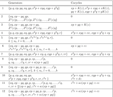
The results of this partial classification of cohomology classes [F], that gives a partial clas-sification of Lie algebras of differential operators g, are summarized in Tables 1 and 2 at the end of this section. The first table gives a 1-cocycle representative for the twelve type I Lie algebras and Table 2 exhibits the results for some general Lie algebras of vector fields among the type III Lie algebras. For these two tables, the classification numbers, given respectively by Lie and Amaldi, sit in the the first column. The second column gives a basis for the Lie algebra h and the third column exhibits the first order differential operators v+ηv for which hF;vi =ηv in not trivial. ηv is taken to be the simplest representative and when the function ηv is trivial, the differential operator is simply the vector field exhibited in the second column. It would be impractical to present the details of the computations in all cases. Furthermore, the arguments are quite similar for all Lie algebra hof vector fields. So, for brevity’s sake, we will only give the details for two of the selected Lie algebras. The chosen examples illustrate well the general process and will give to the reader a good idea of how the calculations proceed in general.
Type I, case 1. This Lie algebra h is spanned by the eight vector fields p, q, xp, yq, xq, yp,x2p+xyqand xyp+y2q. The vector fieldpbelongs to the Lie algebra, hence, as mentioned previously, the functionηpcan be assumed to be zero. The 1-cocycle condition for the pair (p, q) imposes the following restriction
hδ1F;p, qi= (ηq)x−(ηp)y− hF; [p, q]i= (ηq)x ∈ {1}.
Similarly, by considering the pair (p, xp), one concludes that ηxp = cxpx+hxp(y, z), where cxpx can be canceled, without changing the previous functions, by the 0-coboundary of the function Ψxp=cxpx. Then, for the pair (q, xp), the restriction reads as
hδ1F;q, xpi= (ηxp)y−x(ηq)x− hF; [q, xp]i= (hxp(y, z))y−x·cq∈ {1}.
Necessarily, sincehxpdepends only on y and z, the constantcq has to be zero and the function hxp(y, z) is forced to be of the form dxpy+K(z), wheredxp is a constant. Thus, at this point, ηp = 0, ηq= 0 and ηxp=dxpy+K(z).
Consider now the three vector fields yq, xq and yp. If we pair each of them with p and q, from the six 1-cocycle restrictions, one obtains directly the following
ηyq =cyqx+dyqy+kyq(z), ηxq =cxqx+dxqy+kxq(z), ηyp=cypx+dypy+kyp(z).
With the image of the function Ψyq =dyqy, the functionηyq can be reduced toηyq =cyqx+kyq(z) without undoing the previous work. From the restriction associated to the pair (xp, yp), one easily check that
hδ1F;xp, ypi=x(ηyp)x−y(ηxp)x+ηyp=x·cyp+cypx+dypy+kyp(z)∈ {1},
forcing cyp and dyp to be zero andkyp(z) to be a constant function. Similarly, by considering the pair (xp, yq), one obtains that the function x·cyq −y ·dxp must be constant, hence cyq and dxp are zero. To completely determine the functions ηv for these three vector fields, two restrictions, associated to the pairs (xp, xq) and (yp, xq), must be verified. The first imposes thatx(ηxq)x−x(ηxp)y−ηxq =x·cxq−cxqx−dxqy−kxq(z) must be constant. Thus it leaves no choice but to take dxq as the constant zero and kxq(z) as a constant function. Finally, the last restriction forcesy(ηxq)x−x(ηyp)y−ηyq+ηxp=y·cxq−kyq(z)+K(z) to be a constant, hencecxq must be zero whilekxq(z) must be equal, modulo the constant functions, to the functionK(z). Putting together these restrictions, the image of the 1-cocycle F for the first six vector fields of hcan be described as ηp=ηq=ηxq=ηyp= 0 and ηxp=ηyq =K(z). One easily checks that the remaining two restrictions are satisfied.
To determine completely the 1-cocycle F, it remains to find its images for the two vector fields T := x2p+xyq and Q= xyp+y2q. For η
T, three restrictions are needed to reach that ηT = 3xK(z). Indeed, from the pair (p, T), the cocycle condition forces the following equality (ηT)x−2ηxp−ηyq = cT, where cT is a constant. It is not hard to see that ηT must be equal to 3xK(z) +cTx+hT(y, z). From the pair (q, T), we get similarly that ηT = 3xK(z) +cTx+ dTy+kT(z). Finally, the restriction for the pair (xp, T) leads to
x(ηT)x−T(ηxp)−ηT =x·3K(z) +x·cT −(3xK(z) +cTx+dTy+kT(z))∈ {1}.
Hence the constant dT dies out andkT(x) has to be a constant function. Note that, with these 3 restrictions, ηT = 3x(K(z) +cT/3), but, by takingηxp =K(z) +cT/3, one gets the claimed result. By symmetry on x and y, the exact same arguments lead to ηQ = 3yK(z). It is then straightforward to verify that the 1-cocycle F, given by the eight functions
ηp =ηq =ηxq =ηyp = 0, ηxp=ηyq =K(z), ηP = 3xK(z) and ηQ= 3yK(z),
satisfies all the other 1-cocycle conditions. Finally, the Lie algebra g associated to this triple (h,{1},[F]) is the Lie algebra spanned by
p, q, xp+K(z), yp, xq, yq+K(z), x2p+xyq+ 3xK(z), xyp+y2q+ 3yK(z),1 ,
where K(z) can be any function.
Lemma 1. Let i : R2 → R3, (x, y) 7→ (x, y, z) denote the inclusion map and suppose that
h0 ⊂Γ(i∗TR2), meaning that the generators of h0 depend on the variables x and y only. Let h
be a Lie algebra of vector fields on R3 given by h = h
0 ⊕ {r, zr, z2r}. If, for non constant
functions f(x, y) and g(x, y), the vector fields f(x, y)p and g(x, y)q belong to h and if their associated images ηf(x,y)p and ηg(x,y)q depend on x and y only, then
H1(h,F(R3)/{1}) =H1(h0,F(R2)/{1})⊕H1({r, zr, z2r},F(R)/{1}).
Proof . DenoteA:=f(x, y)pandB :=g(x, y)q. From the cocycle restrictions associated to the pairs (A, zir), wherei= 0,1,2, we obtain
hδ1F;A, ziri=A(ηzir)−zi(ηA)z− hF; [A, zir]i=f(x, y)(ηzir)x−0− hF,0i =f(x, y)(ηzir)x∈ {1}.
Since f(x, y) is not constant, (ηzir)x must vanish, hence the functions ηzir depend ony and z. In a similar way, from the restrictions associated to the pairs (B, zir) it is straightforward to conclude that ηzir = hi(z). Finally, for any element v in h0, the function ηv will depend on x and y only. Indeed, since ηzr depends onzonly,
hδ1F;v, zri=v(ηzr)−z(ηv)z− hF; [v, zr]i= 0−z(ηv)z− hF,0i=−z(ηv)z ∈ {1}.
Therefore (ηv)z must be zero, forcing the function ηv to depend onx and y only.
Note thatH1({r, zr, z2r},F(R)/{1}) is already well known. The 1-cocycle F associated the
Lie algebra h={r, zr, z2r} is determined by three functions and the simplest representative is
given by ηr = 0, ηzr = 0 and ηz2
r =dz, for any constant d. Thus, one can use this lemma to simplify some of the computations required in this classification problem. For instance, givenh
the type I Lie algebra of vector fields given by case 10 in Table 1, the Lie algebra of differential operators gbuilt from his obtained from a direct application of this lemma.
Type I, case 10. The Lie algebrah= Span{p, q, xp, yq, xq, yp, x2p+xyq, xyp+y2q, r, zr, z2r} can be decomposed ash0⊕ {r, zr, z2r}whereh0 is the case 1 Lie algebra from the same table. It
was shown in the previous calculations that the functions ηyp and ηxq are zero, hence functions on x and y only. Thus the case 10 Lie algebra, along with its two vector fields yp and xq, satisfies the requirements of the Lemma 1. Therefore, for the vector fields in the algebra h0,
the values of the 1-cocycle depend onx andy only, forcingK(z) to beca constant function. It is then obvious that the 1-cocycle F is defined by eleven functions, were the three non-zero are given by ηT =cx, ηQ = cy and ηz2
r =dx, for c and d any constants. The Lie algebra of first order differential operators g corresponding to this triple is then
g= Span{p, q, xp, yq, xq, yp, x2p+xyq+cx, xyp+y2q+cy, r, zr, z2r+dz,1}.
It should be pointed here thatH1(h,F(M)/{1}) and H1(h,F(M)) can also be determined alternatively using isomorphisms given in [20] and [21]. For the case that interests us, that is H1(h,F(M)/{1}), we fix a base point e and denote i the isotropy subalgebra. Provided the existence of a subalgebra a⊂hwhich is complementary to i, one can show, see [20], that
H1(h,F(M)/{1})∼=H2(h/i).
and ckij are the structure constants of the Lie algebrah, a 1-cocycle inH1(h,F(M)/{1}) will be obtained by solving first the following m(m−1) equations
vi(fj)−vj(fi)−
X
k
ckijfk =αij, for 1≤i < j ≤m.
Once a non unique solution f1, . . . , fm is obtained, the remaining functions fm+1, . . . , fn are determined as the unique solution to them(n−m) equations
vi(fj)−vj(fi)−
X
k
ckijfk =αij, for 1≤i≤m, m+ 1≤j≤n,
with initial conditions
fi(e) = 0 for m+ 1≤i≤n.
Note however that this method can not be applied to all the three dimensional Lie algebras since the existence of the complementary Lie subalgebra is not guaranteed. For instance, the type III case 17A1 can not be treated using the isomorphism. Indeed, for the Lie algebra
h={p, q, xp+zr, yq, x2p+ (2x+az)zr, y2q},
and the base point e = (0,0,0), the isotropy algebra i is generated by the last four elements and the algebra a = {p, q} fails to be complementary, due to the absence of the element r in the Lie algebra. One can easily verify that Z2(h/i) = {α1∧α3, α1∧α5, α2∧α4, α2∧α6} and
B2(h/i) = {α1∧α3, α2 ∧α4}. One can observe at that point that the theorem does not hold,
since the dimension ofH2(h/i) is two while the dimension ofH1(h,F(M)/{1}) was computed to
be three previously. Moreover applying the technique to the 2-cocycleα=c·α1∧α5+d·α2∧α6,
one gets a 1-cocycle that does not satisfies all the conditions that were not considered in the technique detailed above.
2.3 Classif ication of quasi-exactly solvable Lie algebras
of f irst order dif ferential operators and the quantization condition
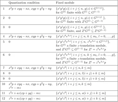
The Lie algebras given in Tables 1 and 2 are the candidates for being quasi-exactly solvable Lie algebras, i.e. we might expect them to admit N a finite dimensional module of smooth functions N. In the investigation for these explicit finite dimensional modules, some new re-strictions are imposed on the 1-cocyclesF. Indeed, as for the quasi-exactly solvable Lie algebras in lower dimensions, it comes out that a finite dimensional module exists only if the values of the functions ηv are taken in a certain discrete set. For this reason, this restriction is named quantization condition. The quasi-exactly solvable Lie algebras and their fixed modules can be found in Tables 3 and 4 for, respectively, the type I and the selected type III Lie algebras. The first column use the same classification numbers as in Tables 1 and 2 and a representative for the non-trivial quantized 1-cocycles is exhibited in the second column. Finally, N, the finite dimensional g-modules of functions are described in the last column. Once again the detailed calculations are repetitive and the essence of the work can be grasped with one or two examples, together with the following general principles.
1. A finite dimensional module for the trivial Lie algebrag={p}is defined as anx-translation module. For instance, any space spanned by a finite set of functions of the form
h= n
X
i=0
along with all their x derivatives, is an x-translation module. This particular case of x-translation module is referred as a semi-polynomial x-translation module. The most general x-translation module is obtained by a direct sum
N =M λ∈Λ
Nλ, Nλ =Nλceλx,
where Nλc are semi-polynomial x-translation modules and the exponents are taken in a finite set Λ, read [9] for more details. Obviously, the y, and the z-translation mod-ules are defined the exact same way.
2. If the Lie algebra g under consideration contains the two differential operators pand xp, the moduleN will be anx-translation module and the operatorxpwill impose extra con-straints. Firstly, all the exponentsλneed be zero. Otherwise, for an non-zero exponentλ, the degree in x of the generating functions in the module Nλc would be unbounded, con-tradicting the finite dimensionality of N. Moreover, if h=Pni=0gi(y, z)xi belongs to the moduleN, the functionxhx also needs to belong to that module. Note that both functions have the same degree in x and are linearly independent ifh is not a monomial. Thus, by an appropriate linear combination of these two functions, one can reduce the number of summands in h. By iterating this process, each generating function can be reduced to a monomial inx. Thus,h=g(y, z)xi where g(y, z) belongs to Gi a finite set of functions in y and z. SinceN is a x-translation module,hx =ig(y, z)xi−1 is also a function in N, hence g(y, z) needs to be also contained in Gi−1. Therefore, the module N decomposes
into the following direct sum
N =Mxigki(y, z), i= 0, . . . , n, k= 0, . . . , li,
where all the functions gik(y, z) belong toGi a finite set and where Gi ⊆Gi−1.
3. Likewise, if a Lie algebrag contains the elementsp,q,xp, and yq, a general finite dimen-sional g-module for this Lie algebra will be at most
N =Mxiyjgi,jk (z), i= 0, . . . , n, j= 0, . . . , m, k= 0, . . . , l(i,j),
where the functionsgi,jk (z) belong toG(i,j), a finite set of functions ofz satisfyingG(i,j)⊆ G(i−1,j)∩G(i,j−1).
A simple method to describe these modules is to represent each generating function xiyjgi,j(z) by a point (i, j), in the Cartesian plane. If a vertex (i, j) belongs to the dia-gram, since N is anxy-translation module, the vertices (i−1, j) and (i, j−1) must also sit in the diagram. To complete the description, a finite set G(i,j) is associated to each of
these vertices, with the same restriction as above. For instance, such module N can be represented by
*
* *
i
** *
* *
j
*
with all the sets G(i,j) being equal to {z, ez}, with the exception of G(3,1) that contains only the functionz. It is then straightforward to verify that this module is indeed
N = Span{0, z, ez, xz, xez, yz, yez, x2z, x2ez, xyz, xyez, y2z,
y2ez, x3z, x3ez, x2yz, x2yez, xy2z, xy2ez, y3z, y3ez, x3yz},
and that it is a g-module for the Lie algebrag={p, xp, y, yq}.
4. If the Lie algebra gcontains the differential operators p,q,xp,yq andyp, from the three previous principles, the generators for a g-module are given by h = xiyjgi,j(z). After applying the operator yp on h, the resulting function reads as ixi−1yj+1gi,j(z). Thus,
iterating this operator, we conclude that all the functions xi−ryj+rgi,j(z) must belong to N, for r ≤i. Since p and q also belong to the algebra, all the functions xaybgi,j(y, z) with a ≤i, b≤ j and a+b≤ c must belong to N. This condition can be expressed by the following inclusion G(i,j) ⊆G(i−1,j)∩G(i,j−1)∩G(i−1,j+1),and observe that the first
set G(i−1,j) can be omitted without affecting the condition. To summarize, the g-module
will be at most
N =Mxiyjgi,jk (z), i= 0, . . . , n, j= 0, . . . , m, k= 0, . . . , l(i,j),
where the functionsgki,j(z) belong toG(i,j), a finite set of functions withG(i,j)⊆G(i−1,j+1)∩
G(i,j−1).
Once again it is possible to represent such module by a diagram along with a set of functions G(i,j) for each vertex of the diagram. The restrictions for these sets areG(i,j)⊆
G(i−1,j+1)∩G(i,j−1) and the conditions on the vertices are slightly different from the one
in the previous example. Indeed, if a vertex (i, j), belongs to the diagram, the two vertices (i−1, j+ 1) and (i, j−1) must also belong to the diagram. Note again that this implies that the vertex (i−1, j) also lies in the diagram. For instance the diagram,
* *
* * *
* *
*
i
** *
* *
*
*
j
* * *
* *
together with twenty appropriate sets of functionsG(i,j) for each vertex, would generate a
g-module for the algebra g={p, q, xp, yq, yp}.
5. Finally, if the elements p,q,xp,yq,ypand xq sit in the Lie algebra under consideration, the module will be at most
N =Mxiyjgki,j(z), i+j = 0, . . . , n, k= 0, . . . , li,j,
where the functions gki,j(z) belong to G(i+j), a finite set of functions with G(l) ⊆G(l−1).
the finite sets G(a,b) are identical and it is therefore well defined to poseG(a,b) =G(a+b). Obviously, sinceN is axy-translation module, the following inclusions holdG(l)⊆G(l−1).
For these modules, the possible diagrams are more restricted and have necessarily the shape of a staircase. Also, instead of assigning one set of functions to each vertex, such a set is coupled to all the vertices having same total degreei+j. For instance, the module represented by the diagram
*
* *
*
i j
* *
*
* * *
* *
* * *
* *
* * *
*
will be completely determined after fixing six sets of function in z. Note that this choice must respect the inclusionG(l)(z)⊆G(l−1)(z), fori= 1, . . . ,5.
Table 1. Cohomology for the type I Lie algebras of vector fields,m={1}.
Generators Cocycles
1 {p, q, xp, yq, xq, yp, x2p+xyq, xyp+y2q} xp+K(z), x2p+xyq+xK(z),
yq+K(z), xyp+y2q+yK(z)
2 {xq, xp−yq, yp, 0
Z1(z)p, . . . , Zl(z)p, Z1(z)q, . . . , Zl(z)q
}
3 {xq, xp−yq, yp, xp+yq, xp+yq+K(z)
Z1(z)p, . . . , Zl(z)p, Z1(z)q, . . . , Zl(z)q
}
4 {p, q, xp, yq, xq, yp, x2p+xyq, xyp+y2q, r} x2p+xyq+cx,xyp+y2q+cy
5 {xq, xp−yq, yp, zkeλlzp, zkeλlzq, r
}, 0
k≤nl, l= 0, . . . , b
6 {xq, xp−yq, yp, xp+yq, xp+yq+cz zkeλlzp, zkeλlzq, r
},k≤nl, l= 0, . . . , b
7 {p, q, xp, yq, xq, yp, x2p+xy, q, xyp+y2q, r, zr} x2p+xyq+cx,xyp+y2q+cy
8 {xq, xp−yq, yp, p, zp, . . . , zlp, 0
q, zq, . . . , zlq, r, zr+a(xp+yq)
}
9 {xq, xp−yq, yp, xp+yq, p, zp, . . . , zlp, 0
q, zq, . . . , zlq, r, zr
},k≤nl, l= 0, . . . , b
10 {p, q, xp, yq, xq, yp, x2p+xyq+cx,xyp+y2q+cy,
x2p+xyq, xyp+y2q, r, zr, z2r
} z2r+dz
11 {xq, xp−yq, yp, p, zp, . . . , zlp, q, zq, . . . , zlq, z2r+az(xp+yq) +cz
r, zr+a
2(xp+yq), z
2r+az(xp+yq)
}
12 {xq, xp−yq, yp, xp+yq, p, zp, . . . , zlp, z2r+az(xp+yq) +cz
q, zq, . . . , zlq, r, zr, z2r+az(xp+yq)
}
Note here that b, l and nl are positive integers, a, c, d, k and λl are arbitrary constants and
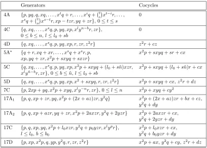
Table 2. Cohomology for some type III Lie algebras of vector fields,m={1}. be a Lie algebra, the parametertneeds to be zero. We then get the Lie algebra 5A∗given in the table.
This set of principles is of great help in the determination of the possibleg-modules N for each Lie algebras of first order differential operators gdescribed in Tables 1 and 2. Depending on the elements contained in the Lie algebra studied, we started our search of g-module based on the general module given in this guideline. Once again, the computations are tedious and it would not be relevant to detail each of them. We will concentrate on the same Lie algebras as in the previous step of this classification problem, that is the type I Lie algebras cases 1 and 10.
Type I, case 1. Since the Lie algebra contains the differential operators p,q, xp, and yp, from the principle (3), the most general moduleN will be spanned by functions of the formh= xiyjgi,j(z), wheregi,j(z) belongs toG(i,j). We now consider the operatorT =x2p+xyq+3xK(z)
in the algebra g and its action on h = xnyagn,a(z) a generator of N with maximal exponent inx. Thus
T[h] =nxn+1yagn,a(z) +axn+1yagn,a(z) + 3K(z)xn+1yagn,a(z) = (n+a+ 3K(z))xn+1yagn,a(z).
Since the exponent inxwas taken to be maximal, this imposes thatK(z) is indeed a constantK equal to −n+a
3 . Symmetrically, by considering Q=xyp+y2q+ 3yK(z) and h =xbymgb,m(z),
a function with maximal exponent in y, the following equality holds K = −b+m
3 . For this to
be possible, we necessarily have n+a = b+m. Consequently, the differential operators xq and ypbelong to the Lie algebra g and the module N is given by the principle (5). Also note that the operators xp and yq force both a and b to be zero. Otherwise xn+1ya−1gn,a(z) and xb−1ym+1gb,m(z) would be in
Table 3. Type I quasi-exactly solvable Lie algebras of differential operators and their fixed modules.
forG(l)a finitez-translation module,
andZiG(l)
⊆G(l−1)forZi=zkeλlzp
6 0 {xiyjzkeλlz
|i+j ≤n, k≤ml, l= 0, . . . , p}, forG(l)a finitez-translation module,
andZiG(l)⊆G(l−1)forZi=zkeλlzp
Note here thatmandnare positive integers.
and the module
N ={xiyjgi,j(z) |i+j≤n, gi,j(z)∈G(i+j)}, where G(l)⊆G(l−1) (8)
is fixed by all the differential operators in g. Therefore it is possible conclude that the Lie algebra
g= Span{p, q, xp, yq, xq, yp, x2p+xyq−nx, xyp+y2q−ny,1},
is quasi-exactly solvable with respect to the finite dimensional g-moduleN.
Type I, case 10. Since the case 10 Lie algebra contains the case 1 Lie algebra, its moduleN will be at most the module given in (8). Observe first that the constantc in the case 10 Lie algebra has to be the negative integer −n. Furthermore, the operator r imposes N to be a z-translation module and the operatorzrforcesG(l)to be generated by monomials. Then, forzm a monomial of maximal degree inG(l), the functionh=xiyl−izm belongs to N. Sincez2r+dz
belongs to the Lie algebra,
z2r+dz[h] =mxiyl−izm+1+dxiyl−izm+1 = [m+d]xiyl−izm+1,
should belong to the g-moduleN. Thus, from the maximality of the degree inz, the constantd has to be the negative integer−m. Since the argument must hold for every setG(l), they will all share the same monomial of maximal degreem. We can therefore conclude that the Lie algebra
g= Span{p, q, xp, yq, xq, yp, x2p+xyq−nx, xyp+y2q−ny, r, zr, z2r−mz,1},
is quasi-exactly solvable with respect to the module
N ={xiyjzk |i+j≤n, k≤m}.
To summarize, a partial classification of quasi-exactly solvable Lie algebras of first order differential operators was accomplished in this section and the description of these Lie algebrasg, along with their g-modules, can be found in Tables 1–4. In principle, it would be possible to achieve a complete classification using similar arguments. However this gigantic work would require a colossal amount of time. Nevertheless this partial classification is a good starting point for seeking new quasi-exactly solvable Schr¨odinger operators in three dimensions. In that scope, the next section is devoted to the description of few new quasi-exactly solvable Schr¨odinger operators.
3
New quasi-exactly solvable Schr¨
odinger operators
in three dimensions
Recall that in the general classification problem, once the quasi-exactly solvable Lie algebras of differential operators g are determined, the next step is to construct second order differential operatorsHthat are locally equivalent to Schr¨odinger operators. Giveng, one of the Lie algebras of first order differential operators obtained in the previous section, we obtain a second order differential operator Hby letting
H= m
X
a,b=1
CabTaTb+ m
X
a=1
CaTa+C0, where Ta∈g, (9)
as illustrated previously. Then, one has to choose the coefficients Cab, Ca, C0 in such a way
are the Frobenius compatibility conditions for the overdetermined system last step in the classification is to verify that the operators are normalizable, i.e. the functions inNe, the module obtained after the gauge transformation, need to be square integrable. These operators will therefore have the property that part of their spectrum can be explicitly computed. We have now in hand a large variety of generating quasi-exactly solvable Lie algebras g. The door is therefore wide open to the construction of numerous new quasi-exactly solvable Schr¨odinger operators in three dimensions. However the Schr¨odinger operators described in this paper are built only from two of these new quasi-exactly solvable Lie algebras: the type III cases 17D and case 5A∗. The reader can therefore see that many more examples can be
constructed using this method together with the results of the previous section.
3.1 Type III, case 17D, (sl(2)×sl(2)×sl(2))
The first two families of normalizable quasi-exactly solvable Schr¨odinger operators displayed in this section are similar to the operator given in the example (1). However, these two examples are more general. Indeed, for these two operators, the type III case 17D quasi-exactly solvable Lie algebra g is spanned by the first order differential operators
p, xp, x2p−mxx, q, yq, y2q−myy, r, zr, z2r−mzz,
where mx,my and mz are non negative integers and the moduleNmxmymz is generated by the (mx+ 1)(my+ 1)(mz+ 1) monomials
xiyjzk where 0≤i≤mx, j≤my and k≤mz.
3.1.1 First example
The first family of operators is constructed with the following choice of coefficients
Cab=
The determinant of the matrix iseg= (1−AC)(x2+ 1)2(By4+ 2(B+ 1)y2+B)(z2+ 1)2 and one easily verifies, forA,B and C positive andAB >1, that the matrix is positive definite on R3.
The operator can therefore be written as
−2H= ∆ +V~ +U,
where ∆ is the Laplace–Beltrami operator related to the metric (10) and where
~
V =−2(x2+ 1)(Amxx+mzz)p−2my(By3+By+y)q−2(z2+ 1)(Cmzz+mxx)r.
From a direct computation, the closure conditions are verified and the gauge factor required to gauge transform Hinto a Schr¨odinger operator H0 is given by
µ= (x2+ 1)−mx2 (By4+ 2(B+ 1)y2+B)
−my
4 (z2+ 1)−mz2 .
Once the transformation is performed, the equivalent operator reads as
−2H0 = ∆ +U,
where the potential of the Schr¨odinger operator−U2 is given by a rational function in y. Note that the same three factors arise in bothµ andeg. This will simplify our computations while testing the square integrability of the functions in Ne. Indeed, a function in Ne is given by h=µxiyjzk where the exponentsi,j andkare smaller or equal tom
x,my andmz respectively. Our aim is to show that the triple integral
ZZZ
R3
(µxiyjzk)2√gdxdydz
is finite. Obviously, it is sufficient to show the convergence of this integral for the monomials of maximal exponent. We can therefore focus on
ZZZ
Using Fubini’s theorem, this triple integral can be factored into the product of three integrals
Z ∞
each of which is easily shown to be convergent. We therefore have in hand a normalizable quasi-exactly solvable Schr¨odinger operator and it is feasible to determine explicitly part of its spectrum.
For instance, if we fix mx = 0, my = 2 and mz = 1, few manipulations lead to the six eigenfunctions of the operator H restricted to N. Indeed, with this choice of parameters, the
g-module is
N ={1, y, y2, z, yz, y2z},
and the transformation matrix to be diagonalized reads as
Once the diagonalization is performed, three different eigenvaluesλ1 =−4−2B,λ2=−2−2B,
and λ3 =−2 + 2B are obtained, each of them having multiplicity two. The six eigenfunctions
are respectively
ψ1,1=y, ψ1,2=yz, ψ2,1 = 1 +y2, ψ2,2=−1 +y2,
ψ3,1=−z+y2z, ψ3,2 =z+y2z.
Consequently, we obtain three multiplicity two eigenvalues of the Schr¨odinger operator H0:
f
As mentioned previously, the metric (10) is positive definite on R3, hence Riemannian, and
one can compute that the Riemann curvature tensor is zero everywhere. The change of variables that leads to a Cartesian coordinate system is given by
X = arctanx, Y =
Z 1
p
By4+ 2(B+ 1)y2+B, Z= arctanz,
where we have some flexibility on B to adjust the roots of the elliptic integral. Note that this operator is a good illustration of the modified Turbiner’s conjecture in three dimensions proved in [6]. Indeed, the generating Lie algebra g is imprimitive and the leaves of the foliation are surfaces, the Riemann curvature tensor is zero and, as expected, the potential is separable since it depends on only one variable.
3.1.2 Second example
With the same representation of Lie algebra by first order differential operators but a different choice of coefficients, one constructs another family of second order differential operators H. Indeed, with
a family of operatorsHis obtained and one easily verifies that all these operators are equivalent to Schr¨odinger operatorsH0. Note that this family of operators is slightly more general than the
family obtained in the first example. However, some of the details are lengthy and are omitted for brevity sake. The induced contravariant metric g(ij) is given by:
and it is positive definite on R3 provided A, B, C, D and β are positive and AB > 1. Its
determinant iseg= (AB−1)(x2+ 1)2(βCy4+ 2βy2+βDy2+y2C+D)(λz2+ 1)2, and the gauge
factor required is the product of three functions in x, y and z respectively. After the gauge transformation the new potential is again a rational function involving only the y variable and the Riemann curvature tensor is null again. The following change of variables leads to Cartesian coordinates
where we have some flexibility on β,C andD to adjust the roots of the elliptic integral Y. However, we do not know if these operators are all normalizable. But, if we fixC =βD, the gauge transformation simplifies and becomes, once again, very similar to the determinant of the metric (11). Indeed
µ= (x2+ 1)−mx2
(β2Dy4+ 2βy2(1 +D) +D)−my4
(λz2+ 1)−mz2
and one verifies, the exact same way as in the previous example, that the functions in Ne are square integrable. Therefore, for any choice of integers mx, my, and mz, one would obtain (mx+ 1)(my+ 1)(mz+ 1) eigenfunctions in the spectrum of the Schr¨odinger operatorH0.
For instance, if we fix λ= 1,β = 5 and the three parameters mx,my and mz to be 1, one gets two eigenvalues, −3 and−7 of multiplicity four, and the following eight eigenfunctions
]
Note that the nodal surfaces can described easily in this coordinate system. Indeed, since µ is always positive, the nodal surfaces are simply the zero loci of polynomials. For these eight eigenfunctions, the surfaces are given by the zeros of degree two factorizable polynomials and one easily gets the following pictures.
−4
For the last example, we consider the type III case 5A∗
quasi-exactly solvable Lie algebra and we fix the parameter s to be one. This Lie algebra g is therefore spanned by the following six first order differential operators
p, q+r, xq+xr, xp, yq+zr, and x2p+xyq+xzr−nx,
and from the Table 4, theg-module of function is given by
wheren,my andmzare non-negative integers. A family of Schr¨odinger operators onR3\{x=y} is obtained from the following choice of coefficients,
Cab=
A 0 0 0 0 0
0 B 0 0 0 0
0 0 C 0 0 0
0 0 0 0 0 0
0 0 0 0 D 0
0 0 0 0 0 0
,
Cc = [0,0, C,0,−2(1 +m)D,0], and C0 = (1 +m)2D,
where the parameters A,B,C, and D are positive. The induced contravariant metric is given by
g(ij)=
Cx2+A 0 0
0 Dy2+B Dyz+B
0 Dyz+B Dz2+B
, (12)
its determinant iseg=BD(Cx2+A)(y−z)2 and the metric is positive definite onR3\{x=y}.
Before performing the gauge transformation the operator reads as
−2H= ∆ + (2Cx−Cmx)p+ (−Dy−2Dmy)q+ (−Dz−2Dmz)r −1/2Cm+ 1/4Cm2+ (1 +m)2D,
and one easily verifies that the operator respects the closure condition. The gauge factor required to obtain a Schr¨odinger operator is
µ= (Cx2+A)1−m
4 (y−z)− 2m−3
2 ,
and once again, contains the same factors as the determinant of the covariant metric. Finally, after the gauge transformation, the Schr¨odinger operator reads as,
−2H0 = ∆ +U,
where U depends on the three variables. Although, it is not known if the functions in Ne are square integrable on the domain R3\{x=y}.
Note that for this example, the scalar curvature is constant and depends on the parameterD while the Riemann curvature tensor is equal to
−1
B(y−z)2dydzdydz.
However, the potential does not seem to be separable.
Acknowledgements
References
[1] Amaldi U., Contributo alla determinazione dei gruppi continui finiti dello spazio ordinario, part I,Giornale di matematiche di Battaglini per il progresso degle studi nelle universita italiane39(1901), 273–316. Amaldi U., Contributo alla determinazione dei gruppi continui finiti dello spazio ordinario, part II,Giornale di matematiche di Battaglini per il progresso degle studi nelle universita italiane40(1902), 105–141. [2] Barut A.O., B¨ohm A., Dynamical groups and mass formula,Phys. Rev. (2)139(1965), B1107–B1112. [3] B¨ohm A., Ne’eman Y., Barut A.O. (Editors), Dynamical groups and spectrum generating algebras, World
Scientific, Singapore, 1988.
[4] B¨ohm A., Ne’eman Y., Dynamical groups and spectrum generating algebras, in Dynamical Groups and Spectrum Generating Algebras, World Scientific, Singapore, 1988, 3–68.
[5] Dothan Y., Gell-Mann M., Ne’eman Y., Series of hadron energy levels as representation of non-compact groups,Phys. Lett.17(1965), 148–151.
[6] Fortin-Boisvert M., Turbiner’s conjecture in three dimensions, J. Geom. Phys., to appear,
math.DG/0612621.
[7] Fulton W., Harris J., Representation theory, Springer-Verlag, 1991.
[8] Gonz´alez-L´opez A., Hurturbise J., Kamran N., Olver P.J., Quantification de la cohomologie des algebres de Lie de champs de vecteurs et fibres en droites sur des surfaces complexes compactes,C. R. Acad. Sci. Paris S´er. I Math.316(1993), 1307–1312.
[9] Gonz´alez-L´opez A., Kamran N., Olver P.J., Lie algebras of first order differential operators in two complex variables,Canadian Math. Soc. Conf. Proc., Vol. 12, Amer. Math. Soc., Providence, R.I., 1991, 51–84.
[10] Gonz´alez-L´opez A., Kamran N., Olver P.J., Normalizability of one-dimensional quasi-exactly solvable Schr¨odinger operators,Comm. Math. Phys.153(1993), 118–146.
[11] Gonz´alez-L´opez A., Kamran N., Olver P.J., New quasi-exactly solvable Hamiltonians in two dimensions,
Comm. Math. Phys.159(1994), 503–537.
[12] Gonz´alez-L´opez A., Kamran N., Olver P.J., Quasi-exactly solvable Lie algebras of first order differential operators in two complex variables,J. Phys. A: Math. Gen.24(1991), 3995–4008.
[13] Gonz´alez-L´opez A., Kamran N., Olver P.J., Quasi-exact solvablility,Contemp. Math.160(1994), 113–139. [14] Gonz´alez-L´opez A., Kamran N., Olver P.J., Real Lie algebras of differential operatord and quasi-exacly
solvable potentials,Philos. Trans. Roy. Soc. London Ser. A354(1996), 1165–1193.
[15] Goshen S., Lipkin H.J., A simple independent particle system having collective properties, Ann. Phys. 6 (1959), 301–309.
[16] Gruber B., Otsuka T. (Editors), Symmetries in science VII: spectrum-generating algebras and dynamic symmetries in physics, Plenum Press, New York, 1993.
[17] Iachello F., Levine R.D., Algebraic theory of molecules, Oxford Univ. Press, Oxford, (1995).
[18] Lie S., Theorie der Transformationsgruppen, Vol. III, Chelsea Publishing Company, New York, 1970.
[19] Milson R., Multi-dimensional Lie algebraic operators, Ph.D. Thesis, McGill University, 1995.
[20] Milson R., Representation of finite-dimensional Lie algebras by first order differential operators. Some local results in the transitive case,J. London Math. Soc. (2)52(1995), 285–302.
[21] Miller W., Jr., Lie theory and special functions, Academic Press, New York, 1968.
[22] Milson R., Richter D., Quantization of cohomology in semi-simple Lie algebras, J. Lie Theory 8(1998), 401–414.
[23] Shifman M.A., Turbiner A.V., Quantal problems with partial algebraization of the spectrum,Comm. Math. Phys.126(1989), 347–365.
[24] Turbiner A.V., Quasi-exactly solvable problems andsl(2) algebras,Comm. Math. Phys.118(1988), 467–474. [25] Ushveridze A.G., Quasi-exactly solvable models in quantum mechanics,Soviet J. Particles and Nuclei 20
(1989), 504–528.