El e c t ro n ic
Jo u r n
a l o
f P
r o b
a b i l i t y Vol. 3 (1998) Paper no. 3, pages 1–59.
Journal URL
http://www.math.washington.edu/˜ejpecp/ Paper URL
http://www.math.washington.edu/˜ejpecp/EjpVol3/paper3.abs.html
The Entrance Boundary of the Multiplicative Coalescent
David Aldous
∗and Vlada Limic
Department of Statistics
University of California
Berkeley CA 94720
e-mail: [email protected]
Abstract The multiplicative coalescent X(t) is al2
-valued Markov process representing co-alescence of clusters of mass, where each pair of clusters merges at rate proportional to product of masses. From random graph asymptotics it is known (Aldous (1997)) that there exists astandardversion of this process starting with infinitesimally small clusters at time−∞. In this paper, stochastic calculus techniques are used to describe all versions (X(t);−∞< t <∞) of the multiplicative coalescent. Roughly, an extreme version is specified by translation and scale parameters, and a vectorc∈l3
of relative sizes of large clusters at time−∞. Such a version may be characterized in three ways: via itst → −∞ behavior, via a representation of the marginal distribution X(t) in terms of excursion-lengths of a L´evy-type process, or via a weak limit of processes derived from the standard multiplicative coalescent using a “coloring” construction.
AMS 1991 subject classifications. 60J50, 60J75
Key words and phrases. Markov process, entrance boundary, excursion, L´evy process, random graph, stochastic coalescent, weak convergence.
Running Head: Coalescent entrance boundary
Submitted to EJP on September 11, 1997. Final version accepted on January 19, 1998.
1
Introduction
1.1
The multiplicative coalescent
Consider the Markov process whose states are unordered collections x =
{xi} of positive real numbers (visualize x as a configuration of clusters of
matter, with xi as the mass of the i’th cluster) and whose dynamics are
described by
for each pair of clusters of masses (x, y), the pair merges at ratexy
into a single cluster of mass x+y. (1)
For a given initial statex(0) with a finite number of clusters, (1) specifies a continuous-time finite-state Markov process. This of course would remain true if we replaced the merger ratexy in (1) by a more general rateK(x, y) (see section 1.6), but the case K(x, y) = xy has the following equivalent interpretation. Regard each cluster i of the initial configuration x(0) as a vertex, and for each pair{i, j}letξi,j be independent with exponential (rate
xi(0)xj(0)) distribution. At timet≥0 consider the graph whose edge-set is
{(i, j) :ξi,j ≤t} and let X(t) be the collection of masses of the connected
components of that graph. Then (X(t),0 ≤ t < ∞) is a construction of the process (1). Aldous [1] shows that we can extend the state space from the “finite-length” setting to the “l2” setting. Precisely, let us represent unordered vectors via their decreasing ordering. Define (l2
ց, d) to be the
metric space of infinite sequences x= (x1, x2, . . .) withx1 ≥x2 ≥. . .≥ 0 and Pix2i < ∞, where d is the natural metric d(x,y) = pPi(xi−yi)2.
Then the “graphical construction” above defines a Markov process (the
multiplicative coalescent) which is a Feller process ([1] Proposition 5) on l2ց and which evolves according to (1). The focus in [1] was on the ex-istence and properties of a particular process, the standard multiplicative coalescent (X∗(t),−∞ < t < ∞), which arises as a limit of the classical
random graph process near the phase transition (see section 1.3). In par-ticular, the marginal distribution X∗(t) can be described as follows. Let (W(s),0≤s <∞) be standard Brownian motion and define
Wt(s) =W(s) +ts−12s2, s≥0. (2)
So Wt is the inhomogeneous Brownian motion with drift t−s as time s. Now construct the “reflected” analog ofWt via
Bt(s) =Wt(s)− min 0≤s′
≤sW
t(s′), s
The reflected processBt has a set of excursions from zero. Then ([1] Corol-lary 2) the ordered sequence of excursion lengths of Bt is distributed as
X∗(t). Note in particular that the total mass P
iXi∗(t) is infinite.
1.2
The entrance boundary
The purpose of this paper is to describe (in Theorems 2 – 4 below) the entrance boundary at time−∞of the multiplicative coalescent. Call a mul-tiplicative coalescent defined for −∞ < t < ∞ eternal. General Markov process theory (see e.g. [7] section 10 for a concise treatment) says that any eternal multiplicative coalescent is a mixture of extreme eternal multipli-cative coalescents, and the extreme ones are characterized by the property that the tail σ-field at time−∞ is trivial. We often refer to different mul-tiplicative coalescents as differentversions of the multiplicative coalescent; this isn’t the usual use of the wordversion, but we don’t have a better word.
Write l3
ց for the space of infinite sequences c = (c1, c2, . . .) with c1 ≥ c2≥. . .≥0 andPic3i <∞. Define parameter spaces
¯
I = [0,∞)×(−∞,∞)×lց3
I+= (0,∞)×(−∞,∞)×lց3 . For c∈l3
ց let (ξj, j ≥1) be independent with exponential (ratecj)
distri-butions and consider
Vc(s) =X
j
cj1(ξj≤s)−c
2
js
, s≥0. (4)
We may regard (cf. section 2.5)Vcas a “L´evy process without replacement”. It is easy to see (section 2.1) that the condition for (4) to yield a well-defined process is precisely the conditionPic3i <∞. Now modify (2,3) by defining, for (κ, τ,c)∈I¯,
f
Wκ,τ(s) =κ1/2W(s) +τ s−12κs2, s≥0 (5)
Wκ,τ,c(s) =Wfκ,τ(s) +Vc(s), s≥0 (6) Bκ,τ,c(s) =Wκ,τ,c(s)
− min
0≤s′≤sW
κ,τ,c(s′), s
≥0. (7)
So Bκ,τ,c(s) is a reflected process with some set of excursions from zero. Now definel0 to be the set ofc∈lց3 such that, for each −∞< τ <∞and eachδ >0,
excursions with length ≥δ (8) (note here κ = 0). If Pic2
i < t, the process W0,t,c(s) has asymptotic
(s → ∞) drift rate t−Pic2i > 0 and hence B0,τ,c ends with an infinite incomplete excursion. Sol0 ⊆l3ց\l2ց. In fact we shall prove (section 5.5)
Lemma 1 l0=l3ց\ l2ց.
Defining
I=I+∪({0} ×(−∞,∞)×l0), we can now state the main results.
Theorem 2 For each(κ, τ,c)∈ I there exists an eternal multiplicative coa-lescentXsuch that for each−∞< t <∞,X(t)is distributed as the ordered sequence of excursion lengths of Bκ,t−τ,c.
Write µ(κ, τ,c) for the distribution of the process X in Theorem 2. Note also that the constant process
X(t) = (y,0,0,0, . . .), −∞< t <∞ (9)
fory≥0 is an eternal multiplicative coalescent: write ˆµ(y) for its distribu-tion.
Theorem 3 The set of extreme eternal multiplicative coalescent distribu-tions is {µ(κ, τ,c) : (κ, τ,c)∈ I} ∪{µˆ(y) : 0≤y <∞}.
Underlying Theorem 3 is an intrinsic characterization of the process with dis-tributionµ(κ, τ,c). From the definition of lց2 , inX(t) = (X1(t), X2(t), . . .) the cluster masses are written in decreasing order, so thatXj(t) is the mass
of thej’th largest cluster. Write
S(t) =X
i
Xi2(t)
Sr(t) =
X
i
Xir(t) , r= 3,4.
Theorem 4 Let (κ, τ,c) ∈ I. An eternal multiplicative coalescent X has distributionµ(κ, τ,c)if and only if
|t|3S3(t) →κ+Pjc3j a.s. ast→ −∞ (10)
t+ 1
S(t) →τ a.s. ast→ −∞ (11)
With this parametrization, the standard multiplicative coalescent has dis-tributionµ(1,0,0). The parametersτ and κ are time-centering and scaling parameters:
if Xhas distributionµ(1,0,c)
thenXe(t) =κ−1/3X(κ−2/3(t−τ)) has distributionµ(κ, τ, κ1/3c) . (13) From (12) we may interpret c as the relative sizes of distinguished large clusters at time−∞. Further interpretations of care addressed in the next two sections, leading to a recipe for constructing the general such process from the standard multiplicative coalescent.
While Theorems 2 – 4 provide concise mathematical characterizations of the processesµ(κ, τ,c), they are not very intuitively informative about the nature of these processes. Indeed we have no appealing intuitive explanation of why excursions of a stochastic process are relevant, except via the proof technique (section 2.3) which represents masses of clusters in the multiplica-tive coalescent as lengths of excursions of certain walks. The technical reason for using Theorem 2 (rather than Theorem 4) as the definition ofµ(κ, τ,c) is that we can appeal to familiar weak convergence theory to establish existence of the multiplicative coalescent with κ = 0, which we do not know how to establish otherwise.
1.3
Relation to random graph processes
The “random graph” interpretation of the standard multiplicative coale-scent X∗ is as follows ([1] Corollary 1). In G(n, P(edge) = 1
n + n4t/3), let Cn
1(t) ≥ C2n(t) ≥ . . . be the sizes of the connected components. Then as n→ ∞, for each fixed t
n−2/3(C1n(t), C2n(t), . . .) →d X∗(t) on l2ց.
Consider c= (c1, . . . , ck,0,0, . . .), and writev =Pic2i. The eternal
multi-plicative coalescent with distributionµ(1,−v,c) arises as the corresponding limit, where in addition to the random edges there are initiallyk“planted” components of sizes⌊cin1/3⌋. (This is a special case of Proposition 7.) From
the viewpoint of random graph asymptotics, it is hard to see which infinite vectors c are appropriate, but in the next section we reformulate the same idea directly in terms of multiplicative coalescents.
roughly for the existence and essential uniqueness of some process like the standard multiplicative coalescent. The following corollary of Theorems 3 and 4 is perhaps the simplest formalization of “essential uniqueness”.
Corollary 5 The standard multiplicative coalescent has the property
X1(t)/S(t)→0 a.s. as t→ −∞.
Any eternal multiplicative coalescent with this property is a mixture of lin-early-rescaled standard multiplicative coalescents.
1.4
The coloring construction
The same idea of “initially planted clusters” can be formulated directly in terms of the multiplicative coalescent. Given a configurationx∈lց2 and a constantc >0, a random configuration COL(x;c) can be defined as follows (see section 5.1 for more details of the following). Imagine distinguishing and coloring atoms according to a Poisson process of rate c per unit mass, so that the i’th cluster (which has mass xi) contains at least one colored
atom with chance 1−e−cxi. Then merge all the clusters containing
col-ored atoms into a single cluster. The notation COL is a mnemonic for “color and collapse”. This operation commutes with the evolution of the multiplicative coalescent; that is, for a version (X(t), t1≤t≤t2), the distri-bution COL(X(t2);c) is the same as the time-t2 distribution of the version started at time t1 with distribution COL(X(t1);c). So given an eternal version X of the multiplicative coalescent, we can define another eternal version COL(X;c) whose marginal distribution at timetis the distribution of COL(X(t);c). For finite c = (c1, . . . , ck) we can construct COL(X;c)
recursively as COL(COL(X; (c1, . . . , ck−1));ck). It turns out that the
con-struction extends toc∈l2ց.
Theorem 6 (a) Let X∗ be the standard multiplicative coalescent, and let c∈ l2ց. Then COL(X∗;c) is the eternal multiplicative coalescent with dis-tribution µ(1,−Pic2
i,c).
(b) Forc∈lց3 ,
µ(1,0,(c1, . . . , ck,0,0, . . .)) →d µ(1,0,c).
(c) Forc∈l0,
This allows us to give a “constructive” description of the entrance boundary. We remark that if c is not in l2ց then COL(X∗;c) does not exist, so one might first guess that (up to rescaling) the entrance boundary consisted essentially only of the processes COL(X∗;c) for c ∈ l2ց. But Theorem 6 says that the process
Yk(t) = COL X∗(t−
k
X
i=1
c2i); (c1, . . . , ck)
!
(14)
has distributionµ(1,0,(c1, . . . , ck)), which as k → ∞ converges weakly to
µ(1,0,c) for allc ∈ l3
ց, not just lց2 . The point is that the increase in l2
-norm caused by the color-and-collapse operation can be compensated by the time-shift. This is loosely analogous to the construction of L´evy processes as limits of linearly-compensated compound Poisson processes. Now by linear rescaling (13) we can defineµ(κ, τ,c) forκ >0, and the final surprise (from the viewpoint of the coloring construction) is that for c ∈ l0 one can let κ→0 to obtain a processµ(0, τ,c).
A related intuitive picture was kindly suggested by a referee. As noted earlier, from (12) we may interpretcas the relative masses of distinguished large clusters in the t → −∞limit. In this limit, these clusters do not in-teract with each other, but instead serve as nuclei, sweeping up the smaller clusters in such a way that relative masses converge. The asymptotic non-interaction allows a comparison where these large clusters may be succes-sively removed, reducing the process to the standard multiplicative coale-scent. In the case where the limit (12) holds with c ∈lց2 this is the right picture, and is formalized in Proposition 41. But as described above, the casec∈l3ցis more complicated.
1.5
Remarks on the proofs
develops the coloring construction, where a central idea (cf. Proposition 41) is that replacingXby COL(X;c) has the effect of appending the vectorcto the vector oft→ −∞ limits in (12). The proof of Theorem 6 is completed in section 5.4.
For at least two of the intermediate technical results (Propositions 14(b) and 30) our proofs are clumsy and we suspect simpler proofs exist.
1.6
General stochastic coalescents
Replacing the merger rate xy in (1) by a general kernel K(x, y) gives a more general stochastic coalescent. Such processes, and their determinis-tic analogs, are the subject of an extensive scientific literature, surveyed for probabilists in [2]. Rigorous study of general stochastic kernels with infinitely many clusters has only recently begun. Evans and Pitman [9] work in the l1 setting, where the total mass is normalized to 1, and give general sufficient conditions for the Feller property. This is inadequate for our setting, where X∗(t) has infinite total mass: Theorem 3 implies
that in l1 the only eternal multiplicative coalescents are the constants. But the l1 setting does seem appropriate for many kernels. For the case K(x, y) = 1 the “standard” coalescent is essentially Kingman’s coalescent [11], say Z = (Z(t); 0 < t < ∞), and it is easy to prove that Z is the unique version satisfying maxiZi(t) → 0 a.s. ast↓ 0. The “additive” case
K(x, y) =x+y seems harder: the “standard” version of the additive coa-lescent is discussed in [9, 4] and the entrance boundary is currently under study.
The stochastic calculus techniques based on (68) used in section 3 can partially be extended to certain other kernels and yield information about the “phase transition” analogous to the emergence of the giant component in random graph theory: see [3].
2
The weak convergence argument
2.1
A preliminary calculation
Let (ξj) be independent with exponential (ratecj) distributions. For fixed
j, it is elementary thatcj1(ξj≤s)−c
2
jsis a supermartingale with Doob-Meyer
decompositionMj(s)−c2j(s−ξj)+, whereMj is a martingale with quadratic
variationhMji(s) =c3jmin(s, ξj). Consider, as at (4),
Vc(s) =X
j
cj1(ξj≤s)−c
2
js
, s≥0.
Forc∈l3ցwe claim thatVcis a supermartingale with Doob-Meyer decom-position
Vc(s) =Mc(s)
−Ac(s) (15)
where
Ac(s) =X
j
c2j(s−ξj)+
and whereMc is a martingale with quadratic variation
hMc
i(s) =X
j
c3jmin(s, ξj). (16)
To verify the claim, it is enough to show that Ac(s) and the right side of (16) are finite. The latter is clear, and the former holds because
E(s−ξj)+≤sP(ξj ≤s)≤s2cj. (17)
Thus the processesWκ,τ,candBκ,τ,cfeaturing in the statement of Theorem 2 are well-defined.
2.2
The weak convergence result
The rest of section 2 is devoted to the proof of the following “domain of attraction” result. Givenx∈l2
ցdefine
σr(x) =
X
i
Proposition 7 For each n ≥ 1 let (X(n)(t);t ≥ 0) be the multiplicative coalescent with initial state x(n), a finite-length vector. Suppose that, as n→ ∞,
σ3(x(n)) (σ2(x(n)))3 →
κ+X
j
c3j (18)
x(jn) σ2(x(n)) →
cj, j≥1 (19)
σ2(x(n)) → 0 (20)
where 0≤κ <∞ and c∈lց3 . If (κ,0,c)∈ I then for each fixed t,
X(n)
1
σ2(x(n)) +t
d
→ Z (21)
whereZis distributed as the ordered sequence of excursion lengths of Bκ,t,c.
Ifκ= 0 and c6∈l0 then the left side of (21) is not convergent.
The special case where c = 0 and κ = 1 is Proposition 4 of [1]. The proof of the general case is similar in outline, so we shall omit some details.
It will be important later that Proposition 7 is never vacuous, in the following sense.
Lemma 8 For any (κ,0,c)∈ I we can choose (x(n)) to satisfy (18 – 20).
Proof. In the case κ > 0 we may (cf. the random graph setting, sec-tion 1.3) take x(n) to consist of n entries of size κ−1/3n−2/3, preceded by entries (c1κ−2/3n−1/3, . . . , cl(n)κ−2/3n−1/3), where l(n)→ ∞ sufficiently slowly. In the case κ = 0 and c ∈ l0, take x(n) to consist of entries (c1n−1/3, . . . , cl(n)n−1/3), where l(n) → ∞ fast enough so that Pil=1(n)c2i ∼
n1/3.
2.3
Breadth-first walk
vertices have a “parent” vertex. Simultaneously we construct the breadth-first walkassociated withX(q).
For each ordered pair (i, j), let Ui,j have exponential(qxj) distribution,
independent over pairs. The construction itself will not involve Ui,i, but
they will be useful in some later considerations. Note that with the above choice of rates
P( edgei↔j appears before time q) = 1−exp(−xixjq) =P(Ui,j ≤xi).
Choosev(1) by size-biased sampling, i.e. vertexv is chosen with probability proportional toxv. Define {v :Uv(1),v ≤xv(1)} to be the set of children of v(1), and order these children asv(2), v(3), . . .so thatUv(1),v(i)is increasing. The children ofv(1) can be thought of as those vertices of the multiplicative coalescent connected tov(1) via an edge by timeq. Start the walk z(·) with z(0) = 0 and let
z(u) =−u+X
v
xv1(Uv(1),v≤u), 0≤u≤xv(1).
So z(xv(1)) =−xv(1)+ X
v child ofv(1) xv.
Inductively, writeτi−1 =Pj≤i−1xv(j). If v(i) is in the same component as v(1), then the set
{v6∈ {v(1), . . . , v(i−1)}:v is a child of one of{v(1), . . ., v(i−1)}} consists ofv(i), . . . , v(l(i)) for somel(i)≥i. Let the children ofv(i) be{v6∈ {v(1), . . ., v(l(i))}: Uv(i),v ≤ xv(i)}, and order them as v(l(i) + 1), v(l(i) + 2), . . .such thatUv(i),v is increasing. Set
z(τi−1+u) =z(τi−1)−u+
X
v child ofv(i)
xv 1(Uv(i),v≤u), 0≤u≤xv(i). (22)
After exhausting the component containingv(1), choose the next vertex by size-biased sampling, i.e. each available vertex v is chosen with probabil-ity proportional to xv. Continue. After exhausting all vertices, the above
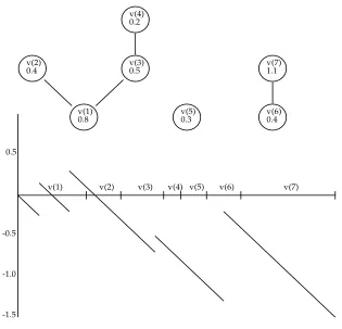
v(1) v(2) v(3) v(4) v(5) v(6) v(7) 0.5
-0.5
-1.0
-1.5
v(1) 0.8 v(2)
0.4 v(3)0.5
v(4) 0.2
v(5)
0.3 v(6)0.4
[image:12.612.149.464.176.479.2]v(7) 1.1
Figure 1
Figure 1 illustrates a helpful way to think about the construction, pictur-ing the successive verticesv(i) occupying successive intervals of the “time” axis, the length of the interval forv being the weightxv. During this time
{v(i), v(i+ 1), . . . , v(j)}, then the walkz(·) satisfies
z(τj) =z(τi−1)−xv(i),
z(u)≥z(τj) onτi−1 < u < τj.
The interval [τj−1, τi] corresponding to a component of the graph has length
equal to the mass of the component (i.e. of a cluster in the multiplicative co-alescent), and this interval is essentially an “excursion above past minima” of the breadth-first walk. This connection is the purpose of the breadth-first walk, and will asymptotically lead to the Theorem 2 description of eternal multiplicative coalescents in terms of excursions ofWκ,τ,c.
2.4
Weak convergence of breadth-first walks
Fix (x(n), n ≥ 1) and t satisfying the hypotheses of Proposition 7. Let (Zn(s),0 ≤ s≤ σ1) be the breadth-first walk associated with the state at time q = σ 1
2(x(n))+t of the multiplicative coalescent started in state x (n). Our first goal is to prove (Proposition 9) weak convergence of 1
σ2(x(n))Zn(s). The argument is an extension of the proof of [1] Proposition 10, in which the termsRn(s) did not arise.
By hypotheses (18 - 20) we may choose m(n) to be an integer sequence which increases to infinity sufficiently slowly that
mX(n)
i=1
(x(in))2 (σ2(x(n)))2 −
mX(n)
i=1 c2i
→0,
mX(n)
i=1
x(in) σ2(x(n)) −
ci
!3
→0, (23)
and σ2(x(n))
mX(n)
i=1
c2i →0. (24)
In the sequel, we will sometimes omitnfrom the notation, and in particular we writeσ2 for σ2(x(n)) and writex forx(n). Consider the decomposition
Zn(s) =Yn(s) +Rn(s) , where Rn(s) = mX(n)
i=1 ˆ xi1{ξn
i≤s}−
x2 i σ2 s ! ,
withξin=β(j) whenv(j) =i, and
ˆ
xi = xi , ifiis not the first vertex in its component
Define
¯ Zn(s) =
1 σ2
Zn(s) =
1 σ2
Yn(s) +
1 σ2
Rn(s) = ¯Yn(s) + ¯Rn(s), say.
Proposition 9 As n → ∞ ( ¯Yn,R¯n) →d (Wfκ,t, Vc), where Vc and Wfκ,t
are independent, and therefore Z¯n →d Wκ,t,c.
First we deal with ¯Yn(s) = ¯Zn(s)−R¯n(s). We can write Yn = Mn+An,
M2
n =Qn+Bn where Mn, Qn are martingales and An, Bn are continuous,
bounded variation processes. If we show that, for any fixed s0,
sup
s≤s0
An(s)
σ2
+κs 2
2 −ts
p
→ 0 (25)
1 σ2
2
Bn(s0)
p
→ κ s0 (26)
1 σ2
2
Esup
s≤s0
|Mn(s)−Mn(s−)|2→0, (27)
then by the standard functional CLT for continuous-time martingales (e.g [8] Theorem 7.1.4(b)) we deduce convergence of ¯Yn toWfκ,t. Note that (27)
is an immediate consequence of (19, 23) and the fact that the largest possible jump ofMn has sizexm(n)+1. Here and below writem form(n). Define
¯
σr=σr− m
X
i=1
xri , r= 2,3,4,5.
It is easy to check that hypotheses (18, 19) and conditions (23, 24) imply
¯
σ2∼σ2 , σ¯3 ¯ σ3
2 →
κ asn→ ∞. (28)
Lemma 11 of [1] extends easily to the present setting, as follows.
Lemma 10
dAn(s) = (−1 + m
X
i=1
x2i/σ2) ds + (t+σ12)(¯σ2−Q2(s)−Q˜2(s)) ds
where, for τi−1 ≤s < τi,
Q2(s) = X
j≤i
x2v(j), Q3(s) = X
j≤i
x3v(j)
˜
Q2(s) = X
j>i,β(j)<s
x2v(j), Q3˜ (s) = X
j>i,β(j)<s
x3v(j),
and all sums above are over vertices j with v(j)∈ {/ 1,2, . . ., m}.
Because 12κs2−ts=Rs
0(κu−t) du, showing (25) reduces, by Lemma 10, to showing
sup
u≤s0
|d(u)| →p 0
where
d(u) =−1 + (t+ 1
σ2)(σ2−Q2(u)− ˜
Q2(u))−tPmi=1x2i
σ2 + (κu−t).
Using (23, 24) and hypotheses (18) and (20), this in turn reduces to proving Lemmas 11 and 12 below. Similarly, (26) reduces to showing
Q3(s0) + ˜Q3(s0) σ3
2
p
→ 0.
Since Q3(s0) ≤ xm+1Q2(s0) and ˜Q3(s0) ≤ xm+1Q˜2(s0), this also follows from Lemma 11 and 12, using (28) and hypothesis (19).
Lemma 11 supu≤s0Q˜2(u)/σ22
p
→ 0.
Lemma 12
sup
u≤s0
1 σ2
2
Q2(u) −σ¯3 σ3 2 u
p
→ 0.
Proof of Lemma 11. Q2˜ (s)≤xm+1Q1˜ (s), where forτi−1≤s < τi
˜ Q1(s) =
X
j>i,β(j)<s
xv(j) ,
and the index j of summation above is not additionally constrained. By (23) and hypothesis (19) we havexm+1/σ2 →0, so it is enough to prove
1 σ2
sup
s≤s0 ˜
This was proved in [1] under the hypothesis x1/σ2 → 0, but examining the argument reveals that our weaker hypothesis (19) is sufficient for the conclusion.
Proof of Lemma 12. This argument, too, is only a slight variation on the one given in [1]. We exploit the fact that the (v(i)) are in size-biased random order. Introduce an artificial time parameterθ, let (Ti) be independent with
exponential(xi) distribution, and consider
D1(θ) = X
j≥1
xj1(Tj≤θ) −σ2θ
D2(θ) = X
j≥m+1
x2j1(Tj≤θ) −σ¯3θ
D0(θ) = 1 σ2
2
D2(θ) − ¯σ3 σ3 2
D1(θ).
Ordering verticesiaccording to the (increasing) values ofTi gives the
size-biased ordering. So the process
1
σ22Q2(τi)− ¯ σ3
σ32τi, i≥0
is distributed as the process (D0(θi), i≥0), where
θi = min{θ:Tj ≤θ for exactlyidifferent j’s from{m+ 1, m+ 2, . . .} }.
In order to prove Lemma 12 it is enough to show that
D(s0) = sup{|D0(θ)| :D1(θ) +σ2θ≤s0} →p 0. (29)
For u = 1,2 the process Du(θ) is a supermartingale, and so by a maximal
inequality ([12] Lemma 2.54.5), forε >0
1
3 εP(sup
θ′≤θ|
Du(θ′)|>3ε)≤E|Du(θ)| ≤
|EDu(θ)|+
q
var Du(θ)
.
Now
|ED2(θ)| = −ED2(θ) = X
j≥m+1
x2j(xjθ+ exp(−xjθ)−1)
≤ X
j≥m+1
x2j (xjθ)2/2
var D2(θ) = X
j≥m+1
x4jP(Tj ≤θ)P(Tj > θ)
≤ X
j≥m+1
x4j (xjθ)
= θσ5¯ .
Similarly
|ED1(θ)| ≤θ2σ3/2; var D1(θ)≤θσ3. (30) Combining these bounds,
1
3εP(sup
θ′
≤θ|
D0(θ′)|>6ε)≤ 1 σ2
2 θ2σ¯
4 2 +θ
1/2¯σ1/2 5
! +σ3
σ3 2
θ2σ 3 2 +θ
1/2σ1/2 3
! .
Setting θ= 2s0/σ2 and using the bounds ¯σ4 ≤xm+1σ3, σ¯5 ≤x2m+1σ3, the bound becomes
O xm+1σ3 σ4
2
+ σ 1/2 3 xm+1
σ25/2 + σ32 σ5 2
+σ 3/2 3 σ27/2
!
and this → 0 using (18,19,20). A simple Chebyshev inequality argument shows that forθ= 2s0/σ2,
P(D1(θ) +σ2θ≤s0)→0,
which together with (29) verifies Lemma 12. 2
We have now shown that ¯Yn →d Wfκ,t. In order to complete the proof of
Proposition 9 we need to show ¯Rn →d Vc, and moreover that ( ¯Yn,R¯n) →d
(Wfκ,t, Vc), whereVcand Wfκ,t are independent. As a preliminary, note thatσ2
2 ≤σ1σ3by the Cauchy-Schwarz inequality, and so by (18,20)
σ1≥σ22/σ3→ ∞. (31)
Define ˜ξinto be the first time of the formτk−1+Uv(k),v(i) for somekwith Uv(k),v(i) ≤xv(k) (this is where we need Uv(i),v(i)). In caseUv(k),v(i) > xv(k) for all k, let ˜ξn
i = σ1 + ξi∗, with ξi∗ d
= exponential((t+ σ1
2)xi), inde-pendent of the walk. By elementary properties of exponentials, ˜ξin has exponential((t+ σ1
2)xi) distribution, and ˜ξ
n
i ,ξ˜jn are independent for i 6=
j , i, j≤n. Obviouslyξn
i ≤ξ˜in and ˜ξni =ξni on the event
By (19) we conclude that ˜ξin →d ξi = exponential(d ci), implying that for
any fixed integerM
M
X
i=1 xi
σ2 1{ξ˜n
i≤u} −
x2i σ2 2 u
!
,0≤u≤s ! d → M X i=1
ci1{ξi≤u}−c
2
iu
,0≤u≤s !
, (33)
asn→ ∞, where the limit (ξi, i≥1) are independent withξi = exponentiald
(rateci),i≥1. We now need a uniform tail bound.
Lemma 13 For each ε >0
lim
M→∞lim supn→∞ P
sup
u≤s
mX(n)
i=M
xi
σ2 1{ξ˜n
i≤u}−
x2i σ2 2 u ! > ε
= 0. (34)
Proof. First split the sum in (34) into
m
X
i=M
[(t+ σ1
2)xi1{ξ˜ni≤u}−(t+
1
σ2) 2x2
iu] + m
X
i=M
[−txi1{ξ˜n
i≤u}+tx
2
iu2+ 2tu x2
i
σ2],
where we recognize the leading term as the supermartingaleV˜c(u) with
˜
c≡(t+ 1
σ2)(xM, xM+1, . . . , xm,0, . . .).
Each remaining term gets asymptotically (uniformly inu) small, asn→ ∞, uniformly inM. For example, for the first one we calculate
E sup
u≤s
t
m
X
i=M
xi1{ξ˜n i≤u}
!
≤t s
m
X
i=M
x2i +s
Pm
i=Mx2i
σ2 →
0 by (20, 24),
and the other two terms are even easier to bound. So it is enough to show
lim
M→∞lim supn→∞ P supu≤s
m X
i=M
(t+σ1
2)xi1{ξ˜ni≤u} −(t+
1
σ2) 2x2
iu > ε ! = 0.
(35) For (M˜c, A˜c) defined in (15), estimates (16, 17) give
E(M˜c)2(s)
≤
m
X
i=M
(t+σ1 2)
3x3
i s , EA˜c(s)≤ m
X
i=M
(t+σ1 2)
3x3
i s2.
Hypotheses (18 – 20) and conditions (23, 24) imply
lim
n→∞
m
X
i=M
(t+ σ1 2)
3x3
i =
∞
X
i=M
and now a standard maximal inequality application yields (35). 2
Lemma 13 and (33) imply, by a standard weak convergence result ([6] Theorem 4.2), m X i=1 xi σ2 1{ξ˜n
i≤s}−
x2i σ2 2 s
!
d
→ Vc(s). (36)
Because ( ˜ξin, i < m) is independent ofYn(s), we have joint convergence
¯ Yn(s),
m
X
i=1 xi
σ21{ξ˜ni≤s}−
x2i σ22s
!!
d
→ (Wfκ,t, Vc(s)), (37)
with independentWfκ,t and Vc(s). To complete the proof of Proposition 9 it is enough to show that
sup
u≤s
m X i=1 x i σ2 1{ξ˜n
i≤u}−
ˆ xi
σ2 1{ξn
i≤u}
= supu≤s
m X i=1 xi σ2 1{ξn
i<ξ˜ni≤u}
= m X i=1 xi
σ21{ξin<ξ˜in≤s} (38)
p
→ 0. (39)
For the event {ξin < ξ˜in ≤ s} to occur at some random time U ≤ s the walk must exhaust some finite number of components ending with a vertex v(J), and then v(J+ 1) must be i. Since v(J + 1) is chosen by size-biased sampling,
P(v(J+ 1) =i|U, J) = xi σ1−U ≤
xi
σ1−s
on{U ≤s}a.s..
In other words P(ξn
i < ξ˜in≤s) ≤ σ1x−is on {U ≤s}. So the expectation of (38) equals m X i=1 xi σ2
P(ξin<ξ˜in≤s)≤
m
X
i=1 xi
σ2 · xi
σ1−s ≤ 1 σ1−s →
0 ,
by (31).
2.5
Properties of the L´
evy-type limit process
in (l2ց, d) to the excursions of reflectedWκ,t,c, which is defined to be Bκ,t,c. This will be done in section 2.6. As a preliminary, we need the following properties of the limit process, which were routine, and hence not explicitly displayed, in the “purely Brownian” c = 0 setting of [1]. In principle one should be able to prove Lemma 1 also directly from the definition, but we are unable to do so.
Proposition 14 Let(κ, t,c) ∈ I and write W(s) =Wκ,t,c(s) and B(s) = Bκ,t,c(s). Then
(a)W(s) → −∞p ass→ ∞. (b) P(B(s) = 0) = 0, s >0.
(c) max{y2−y1 : y2 > y1 ≥s0,(y1, y2) is an excursion of B(·)}
p
→ 0 as
s0 → ∞.
(d) With probability1, the set{s:B(s) = 0} contains no isolated points.
The proof occupies the rest of section 2.5. As at (15) write
W(s) =κ1/2W∗(s) +ts−1 2κs
2+Mc(s)
−Ac(s), (40)
whereW∗ is a standard Brownian motion. It follows easily from (16) that
s−1Mc(s)
→0 a.s. as s→ ∞. (41)
Moreover (1−ξi
s)+c2i ↑c2i for alli, so by the monotone convergence theorem
Ac(s) s =
X
i
1−ξi
s
+
c2i →Xc2i ≤ ∞ a.s..
Recall that Pic2i = ∞ if κ = 0. Since of course s−1W∗(s) → 0 a.s., representation (40) impliess−1W(s)→ −∞ a.s., which gives assertion (a).
Assertion (c) is true by definition of l0 in the case κ = 0. If κ > 0 we may assumeκ= 1 by rescaling. Restate (c) as follows: for eachε >0
number of (excursions ofB with length>2ε) <∞ a.s. (42)
Fixε >0 and define eventsCn={sups∈[(n−1)ε,nε](W((n+1)ε)−W(s))>0}. For t1, t2 ∈ R, write t1 ∼ t2 if both t1 and t2 are straddled by the same excursion ofB. Note that{(n−1)ε6∼nε∼(n+ 1)ε} ⊂Cn, so it suffices to
showP(Cn i.o.) = 0. In fact, by (41) it is enough to show
X
n≥s0/ε
whereCs0 ={sup
s≥s0|M(s)/s| ≤
ε2
4}. From (40) we get Cn⊆ { sup
s∈[(n−1)ε,nε]
W∗(ε(n+ 1))−W∗(s)>(−2tε)∧(−εt)
+ε 2
2(2n+ 1) +A((n+ 1)ε)−A(nε)−s∈[(nsup−1)ε,nε]M((n+ 1)ε)−M(s)}.
Considernlarge enough so thatn−1≥s0/εand 2tε <(2n+ 1)ε2/8. Then, while onCs0,
sup
s∈[(n−1)ε,(n+1)ε]
M(s) (2n+ 1)ε
<
ε2 8 ,
and so
Cn∩Cs0 ⊆
(
sup
s∈[(n−1)ε,nε]
W∗(ε(n+ 1))−W∗(s)≥ ε 2
8 (2n+ 1) )
.
Since the increment distribution ofW∗ doesn’t change by shifting time, nor by reversing time and sign,
P(Cn∩Cs0) ≤ P( sup s∈[ε,2ε]
W∗(s)> ε 2
8 (2n+ 1))
≤ P(W∗(ε)> ε 2
16(2n+ 1)) +P( sups∈[0,ε]W
∗(s)> ε2
16(2n+ 1))
≤ ε3(2512n+ 1)2, by a maximal inequality.
This establishes (43) and hence assertion (c).
The proofs of (b) and (d) involve comparisons with L´evy processes, as we now discuss. Given (κ, t,c)∈ I, one can define the L´evy process
L(s) =κ1/2W∗(s) +ts+X
i
(ciNi(s)−c2is)
whereW∗ is standard Brownian motion and (Ni(·), i≥1) are independent
Poisson counting processes of ratesci. Clearly
W(s)≤L(s), s≥0. (44)
By a result on L´evy processes (Bertoin [5] Theorem VII.1)
This is already enough to prove (d), as follows (cf. [5] Proposition VI.4). For a stopping timeSforW(·), the incremental process (W(S+s)−W(S), s≥0) conditioned on the pre-S σ-field is distributed asWκ,t′
,c′(s) for some random t′,c′. Applying this observation toSr= inf{s≥r :W(s) = inf0≤u≤sW(u)},
and then applying (44,45) toWκ,t′
,c′(s) and the corresponding L´evy process, we see that Sr is a.s. not an isolated zero. This fact, for all rationalsr,
implies (d).
It remains to prove assertion (b). We first do the (easy) caseκ >0. Fix s, look at the process just before time s, and Brownian-scale to define
Wε(u) =ε−1/2(W(s−uε)−W(s)), 0≤u≤1.
We claim that
Wε(·) →d κ1/2W∗(·) asε→0. (46)
Clearly κ1/2W∗ arises as the limit of the κ1/2W∗(u) +tu− 12κu2 terms of W, so it is enough to show
(ε−1/2(Vc(s
−uε)−Vc(s)), 0
≤u≤1) →d 0 as ε→0. (47)
Now the contribution to the left side of (47) from the (cj1(ξj≤u)−c
2
ju) term
ofVc is asymptotically zero for each fixedj; and as in section 2.1 a routine variance calculation enables us to bound sup0≤u≤1ε−1/2(Vc(s−uε)−Vc(s)) in terms of Pjc3j. This establishes (47) and thence (46). Combining (46) with the fact that inf0≤u≤1κ1/2W∗(u)<0 a.s. impliesP(infs−ε≤u≤sW(u)<
W(s))→1 as ε→0. Thus P(W(s) = infu≤sW(u)) = 0, which is (b).
It remains to prove assertion (b) in the case κ = 0. Recall that in this case Pic2
i =∞ and
P
ic3i <∞. By ([5] Theorem VII.2 and page 158) the
analog of (b) holds forL(·): for fixeds0,
P(L(s0) = inf 0≤u≤s0
L(u)) = 0. (48)
To prove (b) we will need an inequality in the direction opposite to (44): this will be given at (50).
Fixs0. Define a mixture of L´evy processes by
Qm(s) = t− m
X
i=1 c2i
!
s+ X
i≥m+1
ci1AiMi(s)−c
2
is
converges by comparing with the sum defining L(s), because E(Ni(s) −
1AiMi(s)) = O(c
2
i) as i → ∞. Applying to (Qm) the L´evy process result
(48),
P
Qm(s0) = inf 0≤u≤s0
Qm(u)
= 0. (49)
We shall show that the processes (Q2m(u),0≤u≤s0) and (W(u),0≤u≤
s0) can be coupled so that
P(Q2m(s0)−Q2m(u)≤W(s0)−W(u) for all 0≤u≤s0)→1 as m→ ∞. (50) Then (49,50) imply
P
W(s0) = inf 0≤u≤s0
W(u)
= 0
which is assertion (b).
We shall need the following “thinning” lemma.
Lemma 15 Given s0, λ, λi, i ≥ 1 such that λ ≤ λie−λis0, let (ξi, i ≥ 1)
be independent, with ξi having exponential(λi) distribution. Then we can
construct a rate-λ Poisson point process on[0, s0]whose points are a subset of (ξi,1≤i≤V) where V −1 has Poisson(λs0) distribution.
Proof. If ξ1 > s0, set V = 1. If ξ1 = s ≤ s0, toss a coin independently, with λλe−λs
1e−λ1s probability of landing heads. If tails, delete the point ξ1 and set V = 1. If heads, the point ξ1 becomes the first arrival of the Poisson process. Next consider the interval I1 = [ξ1, s0] = [s, s0] and the point ξ2. Ifξ2 6∈I1, set V = 2. Else, the pointξ2 =s+t becomes the second arrival of the Poisson process with probability λe−λt
λ2e−λ2 (s+t). Continue in the same manner. 2
Recall that, in the present κ= 0 setting,
W(s) =ts+X
i
(ci1(ξi≤s)−c
2
is)
where ξi has exponential(ci) distribution. Write (ξi,j, j ∈Ji) for the set of
points of Mi(·) in [0, s0] if Ai occurs, but to be the empty set if Ai does
not occur. We seek to couple the points (ξi,j,2m < i < ∞, j ∈ Ji) and
the points (ξi,1≤i <∞) in such a way that ξi,j =ξh(i,j) for some random h(i, j)≤isuch that the values{h(i, j) :i >2m, j∈Ji}are distinct. Say the
a coupling of (Q2m(u),0 ≤u ≤ s0) and (W(u),0 ≤ u ≤ s0) such that the inequality in (50) holds. So it will suffice to show that the probability of a successful coupling tends to 1 as m → ∞. The construction following involves ξi for i ≥ m. Since we are proving the m → ∞ limit assertion
(51), we may suppose thatcie−cis0 is non-increasing ini≥mand thatci is
sufficiently small to satisfy several constraints imposed later.
FixM >2m. We work by backwards induction onk=M, M −1, M − 2, . . . ,2m+ 1. Suppose we have defined a joint distribution of (ξi,j, M ≥
i ≥ k+ 1, j ∈ Ji) and (ξi, M ≥ i ≥ k+ 1−D(k+ 1)), for some random
D(k+ 1)≥0. For the inductive step, ifAkdoes not occur then the setJk is
empty, so the induction goes through forD(k) = (D(k+1)−1)+. IfAkdoes
occur, we appeal to Lemma 15 to construct the points (ξk,j, j ∈ Jk) as a
subset of the points (ξi, k−D(k+1)≥i≥k−D(k)), where D(k)−D(k+1)
has Poisson(¯cks0) distribution and is independent ofD(k+ 1). We continue this construction until
TM = max{k < M :D(k)≥k−m},
after which point the “λ≤λi” condition in the Lemma 15 might not hold.
ProvidedTM <2m we get a successful coupling. Thus it is enough to prove
lim
m→∞lim supM→∞ P(TM ≥2m) = 0. (51)
By construction, (D(k) :M ≥k≥TM−m) is the non-homogeneous Markov
chain specified by D(M+ 1) = 0 and
D(k) = (D(k+ 1)−1)+ on an event of probability min(1,2cks0);
otherwiseD(k)−D(k+ 1) has Poisson(¯cks0) distribution . (52)
We analyze this chain by standard exponential martingale techniques.
Lemma 16 There exist θ > 1 and α > 0 such that, provided ck is
suffi-ciently small,
E(θD(k)|D(k+ 1) =d)≤θdexp(−αck), d≥1.
Proof. We may take 2cks0 <1, and then the quantity in the lemma equals
2cks0θd−1 + (1−2cks0)θdexp((θ−1)¯cks0).
Since ¯ck≤ck, we obtain a bound θdf(ck) where
Sof(0) = 1 and
f′(0) = 2s0(θ−1−1) + (θ−1)s0 = −2s0
15 , choosingθ= 6/5. Soα=s0/8 will serve. 2
Now fix i and consider ζi = max{j ≤i:D(j) = 0}. Lemma 16 implies
that the process
Λ(k) =θD(k)exp(α(ci−1+. . .+ck)), i≥k≥ζi
is a supermartingale. On the event{TM ≥max(2m, ζi)}we have
Λ(TM)≥θTM−mexp(α(ci−1+. . .+cTM))≥θ
mexp(α(c
i−1+. . .+c2m))
the second inequality because we may assume c2m is sufficiently small that
exp(αc2m)< θ. Since Λ(i) =θD(i), the optional sampling theorem implies
P(i≥TM ≥max(2m, ζi)|D(i))≤θD(i)−me−α(ci−1+...+c2m) on{D(i)≥1}
and the conditional probability is zero on{D(i) = 0}. From the transition probability (52) for the step fromi+ 1 toi,
E(θD(i)1(D(i)≥1)|D(i+ 1) = 0) = exp((θ−1)¯cis0)−exp(−c¯is0) ≤ θ¯cis0 ≤θcis0.
Combining with the previous inequality,
P(i≥TM ≥max(2m, ζi)|D(i+ 1) = 0)≤θ−me−α(ci−1+...+c2m) θcis0. (53)
By considering the smallesti≥TM such thatD(i+ 1) = 0,
P(TM ≥2m) = M
X
i=2m
P(D(i+ 1) = 0, i≥TM ≥max(2m, ζi))
≤
M
X
i=2m
P(i≥TM ≥max(2m, ζi)|D(i+ 1) = 0).
Substituting into (53), to prove (51) it suffices to prove
θ−m ∞
X
i=2m
In fact the sum is bounded inm, as we now show. For integer q ≥0 write A(q) = {i :q ≤ ci−1+. . .+c2m < q+ 1}. Then (since we may take each
ci <1) we have Pi∈A(q)ci ≤2. So
X
i∈A(q)
ciexp(−α(ci−1+. . .+cm))≤2 exp(−αq)
and the sum overq is finite, establishing (54).
2.6
Weak convergence in
l
2The remainder of the proof of Proposition 7 follows the logical structure of the proof of Proposition 4 in [1]. We are able to rely on the theory of size-biased orderings for random sequences inl2
ց and convergence, developed in
[1], section 3.3, which we now repeat.
For a countable index set Γ write l2+(Γ) for the set of sequences x = (xγ;γ∈Γ) such that eachxγ≥0 andPγx2γ<∞. Write ord :l+2(Γ)→lց2 for the “decreasing ordering” map.
Given Y = {Yγ : γ ∈ Γ} with each Yγ > 0, construct r.v.’s (ξγ) such
that, conditional onY, the (ξγ) are independent andξγ has exponential(Yγ)
distribution. These define a random linear ordering on Γ, i.e. γ1 ≤ γ2 iff ξγ1 ≤ξγ2. For 0≤a <∞define
S(a) =X{Yγ :ξγ < a}. (55)
Note that
E(S(a)|Y) =X
γ
Yγ(1−exp(−aYγ))≤a
X
γ
Yγ2.
So if Y ∈ l+2(Γ) then we have S(a) < ∞ a.s.. Next we can define Sγ =
S(ξγ)<∞and finally define thesize-biased point process(SBPP) associated
withY to be the set Ξ ={(Sγ, Yγ) :γ ∈Γ}. So Ξ is a random element of
M, the space of configurations of points on [0,∞)×(0,∞) with only finitely many points in each compact rectangle [0, s0]×[δ,1/δ]. Note that Ξ depends only on the ordering, rather than the actual values, of theξ’s. Writingπ for the “project onto they-axis” map
π({(sγ, yγ)}) ={yγ} (56)
we can recover ordY from Ξ via ordY= ord π(Ξ).
Proposition 17 ([1] Proposition 15) Let Y(n) ∈ l2+(Γn) for each 1 < n≤ ∞, and letΞ(n) be the associated SBPP. Suppose
Ξ(n) →d Ξ(∞), (57)
where Ξ(∞) is a point process satisfying
sup{s: (s, y)∈Ξ(∞) for some y}=∞ a.s. (58)
if (s, y)∈Ξ(∞) then X{y′ : (s′, y′)∈Ξ(∞), s′< s}=s a.s. (59)
max{y: (s, y)∈Ξ(∞) for some s > s0}
p
→ 0 as s0 → ∞. (60)
ThenY(∞)= ord π(Ξ(∞)) is in lց2 , andord Y(n) →d ordY(∞).
Let Ξ(∞) be the point process with points
{(l(γ),|γ|), γan excursion of Bκ,t,c },
wherel(γ) and|γ|are the leftmost point and the length of an excursion γ. In the setting of Proposition 7, let Y(n) be the set of component sizes of the multiplicative coalescent at time t+ 1/σ2. If the k’th component of the breadth-first walk consists of vertices {v(i), v(i+ 1), . . ., v(j)}, let l(n, k) = τi−1 and C(n, k) = τj −τi−1 be the leftmost point and the size of the corresponding excursion. Let Ξ(n) be the point process with points
{(l(n, i), C(n, i)) : i ≥ 1}. Since the components of the breadth-first walk are in size-biased order, Ξ(n) is distributed exactly as the SBPP associated with Y(n). So the proof of convergence (21) in Proposition 7 will be com-pleted when we check the hypotheses of Proposition 17. But (58,59,60) are direct consequences of Proposition 14(a,b,c). Moreover, the weak conver-gence ¯Zn →d W given by Proposition 9, combined with the property of
Proposition 14(d), implies by routine arguments (cf. [1] Lemma 7) the weak convergence (57) of starting-times and durations of excursions: we omit the details.
To establish the “non-convergence” assertion of Proposition 7, suppose κ= 0 andc∈l3ց\l0. So for somet and δ,
P(B0,t,chas infinitely many excursions of length > δ)> δ (61)
the paragraph above show that for someω(n)→ ∞
lim inf
n P
X(n)
1
σ2(x(n))+t
contains≥ω(n) clusters of size≥δ
> δ
(62) implying non-convergence inl2ց.
3
Analysis of eternal multiplicative coalescents
This section is devoted to the proof of
Proposition 18LetXbe an extreme eternal multiplicative coalescent.Then eitherX is a constant process (9) or else
|t|3S3(t) →a a.s. ast→ −∞ (63) t+ 1
S(t) →τ a.s. ast→ −∞ (64)
|t|Xj(t) →cj a.s. ast→ −∞, eachj ≥1 (65)
where c∈lց3 , −∞< τ <∞,a >0 and Pjc3j ≤a <∞.
3.1
Preliminaries
As observed in [1] section 4, whenX(0) =xis finite-length, the dynamics (1) of the multiplicative coalescent can be expressed in martingale form as fol-lows. Letx(i+j)be the configuration obtained fromxby merging thei’th and j’th clusters, i.e. x(i+j)= (x1, . . . , xu−1, xi+xj, xu, . . . , xi−1, xi+1, . . . , xj−1 , xj+1, . . .) for someu. WriteF(t) =σ{X(u);u≤t}. Then
E(∆g(X(t))|F(t)) =X
i
X
j>i
Xi(t)Xj(t)
g(X(i+j)(t))−g(X(t))dt (66)
for all g : lց2 → R (for all g because there are only finitely many possible states). Of course, our “infinitesimal” notation E(∆Y(t)|F(t)) = A(t)dtis just an intuitive way of expressing the rigorous assertion thatM(t) =Y(t)− Rt
the finite-length setting, using the Feller property ([1] Proposition 5). In this way we finesse the issue of proving the strong Markov property in the l2
ց-valued setting, or discussing exactly which functionsgsatisfy (66) in the
l2ց-valued setting.
Because a merge of clusters of sizesxi and xj causes an increase inS of
size (xi+xj)2−xi2−x2j = 2xixj, (66) specializes to
E(∆f(S(t))|F(t)) =X
i
X
j>i
Xi(t)Xj(t) (f(S(t) + 2Xi(t)Xj(t))−f(S(t)))dt
(67) which further specializes to
E(∆S(t)|Ft) = 2
X
i
X
j>i
Xi2(t)Xj2(t)dt= S2(t)−X
i
Xi4(t) !
dt. (68)
3.2
Martingale estimates
In this section we give bounds which apply to the multiplicative coalescent (X(t), t≥0) with arbitrary initial distribution.
Lemma 19 LetT = min{t≥0 :S(t)≥2S(0)}. Then
E
Z T
0
(S(t)−X12(t))dt≤5.
Proof. AssumeX(0) is deterministic, and writes(0) =S(0). SincePiXi4(t)
≤X2
1(t)S(t), by (68)
E(∆S(t)|Ft)≥S(t)(S(t)−X12(t)) dt≥s(0)(S(t)−X12(t))dt.
By the optional sampling theorem,
ES(T)−s(0)≥s(0)E
Z T
0
(S(t)−X12(t)) dt.
But S(T−)≤2s(0) and S(T)−S(T−)≤2X12(T−) ≤2S(T−), so S(T)≤ 6s(0), establishing the inequality asserted in the Lemma. 2
Lemma 20 ([1] Lemma 19) Write Z(t) =t+S1(t). Then
0≤E(∆Z(t)|F(t))≤ S4(t) S2(t) +
2(S3(t))2 S3(t)
!
and
var (∆Z(t)|F(t))≤ 2(S3(t)) 2
S4(t) dt. (70)
Lemma 21 DefineY(t) = logS3(t)−3 logS(t). Then (i)|E(∆Y(t)|F(t))| ≤15X12(t)dt
(ii)var (∆Y(t)|F(t))≤36X2 1(t)dt.
Proof. Write S2(t) for S(t). By (66) E(∆Y(t)|F(t)) equals dt times the following expression, where we have dropped the “t”:
X
i
X
j>i
XiXj[log(S3+ 3Xi2Xj+ 3XiXj2)−logS3]
−3X
i
X
j>i
XiXj[log(S2+ 2XiXj)−logS2].
Using the inequality|log(a+b)−loga− ba| ≤ 2ba22 fora, b >0, we see that
|E(∆Y(t)|F(t))|is bounded by dttimes 1 S3 X i X j>i
XiXj(3Xi2Xj+ 3XiXj2) −
3 S2 X i X j>i
2Xi2Xj2 (71) +X i X j>i
XiXj
(3Xi2Xj+ 3XiXj2)2
2S2 3
+ 3X
i
X
j>i
XiXj
(2XiXj)2
2S2 2
. (72)
The quantity (72) is at most
9 2 S5 S3 +S 2 4 S2 3 ! +3S
2 3 S2
2
(73)
which is bounded by 12X12, using the fact Sr+1/Sr ≤X1. The quantity in (71) equals S3|Z|
2S3, where Z = X
i
X
j6=i
X
k
Xi3Xj2Xk2−X
i
X
j
X
k6=j
Xi3Xj2Xk2
= −S5S2+S3S4,
and so the quantity in (71) equals 3S4
S2 −
S5
S3
≤ 3X2
1. Combining these bounds gives (i). For (ii), note that var (∆Y(t)|F(t)) equals dt times an expression bounded from above by
X
i
X
j>i
+9X
i
X
j>i
XiXj[log(S2+ 2XiXj)−logS2]2.
Since (log(a+b)−loga)2≤(b/a)2fora, b >0, we repeat the argument via (72,73), with slightly different constants, to get the bound
9 S5 S3
+S 2 4 S2 3
! +18S
2 3 S2
2 ≤
36X12. 2
Now imagine distinguishing some cluster at time 0, and following that distinguished cluster as it merges with other clusters. Write X∗(t) for its
size at timet. It is straightforward to obtain the following estimates.
Lemma 22 E(∆X∗(t)|F(t)) = (X∗(t)S(t)−X∗3(t))dt
var (∆X∗(t)|F(t))≤X∗(t)S3(t)dt.
Our final estimate relies on the graphical construction of the multiplicative coalescent, rather than on martingale analysis.
Lemma 23
P(S(t)≤t X1(0), X2(t)≥δ|X(0))≤δ−2tX1(0) exp(−δtX1(0)).
Proof. We may assume X(0) is a non-random configuration x(0). We may constructX(t) in two steps. First, let Y(t) = (Yj(t), j ≥1) be the state at
time t of the multiplicative coalescent with initial state (x2(0), x3(0), . . .). Second, for eachj ≥1 merge the clusterYj(t) with the cluster of sizex1(0)
with probability 1−exp(−tx1(0)Yj(t)), independently asj varies. WriteN
for the number of j such that Yj(t) ≥ δ, and let M ≤ N be the number
of these j which do not get merged with the cluster of size x1(0). Since S(t)≥N δ2, the probability we seek to bound is at most
P(N ≤δ−2tx1(0), M ≥1) ≤ P(M ≥1|N ≤δ−2tx1(0)) ≤ E(M|N ≤δ−2tx1(0)) ≤ δ−2tx1(0) exp(−tx1(0)δ).
3.3
Integrability for eternal processes
Proposition 24LetXbe an extreme eternal multiplicative coalescent.Then eitherX is a constant process (9) or else
lim sup
t→−∞ |
Z 0
−∞
X12(t)dt <∞ a.s. (75)
and Z
0
−∞
S2(t)dt <∞ a.s. . (76)
Proof. By extremality
lim sup
t→−∞ |
t|X1(t) =C a.s. (77)
for some constant 0≤ C ≤ ∞. Suppose C =∞. Fix a large constantM and define
Tn= inf{t≥ −n:|t|X1(t)≥M}.
Applying Lemma 23 to (X(Tn+u), u ≥ 0) and t = −Tn, on the event
{Tn<0}, gives
P(Tn<0, S(0)≤ |Tn|X1(Tn), X2(0)≥δ)
≤δ−2E|Tn|X1(Tn) exp(−δ|Tn|X1(Tn)).
The supposition C = ∞ implies thatP(Tn <0,|Tn|X1(Tn) ≥ M) → 1 as
n→ ∞, and so
P(S(0)≤M, X2(0)≥δ)≤δ−2 sup{yexp(−δy) :y≥M}. (78)
LettingM → ∞we see P(X2(0)≥δ) = 0. But δ is arbitrary, and soX(0) consists of just a single cluster. The same argument applies toX(t) for each t, and hence X is a constant process. So now consider the case C <∞, i.e. where (74) holds. Then (75) follows immediately. So we can defineU >−∞ by
Z U
−∞X 2
1(t)dt= 1.
Note that a.s. limt→−∞S(t) = 0. Otherwise we would have S(t) → s∗, s∗ >0 a constant by extremality, and Lemma 19 would giveX
1(t)→ √s∗, contradicting (74). Now define
e
Tm= inf{t:S(t)≥2−m}, m= 1,2, . . .
so thatP(Tm>−∞) = 1 for allmand Tm↓ −∞. Using Lemma 19,
E
Z Tm
Tm+1
(S(t)−X12(t))dt≤5.
BecauseS(t)≤2−m on Tm+1≤t < Tm,
E
Z Tm
Tm+1
S2(t)dt≤2−mE
Z Tm
Tm+1
S(t)dt≤2−m 5 +E
Z Tm
Tm+1
X12(t)dt !
.
Summing overm,
E Z T1
−∞
S2(t)dt≤5 +E Z T1
−∞
X12(t)dt≤6
establishing (76).
3.4
Proof of Proposition 16
We quote a version of the L2 maximal inequality and the L2 convergence theorem for (reversed) martingales.
Lemma 25 Let (Y(t);−∞ < t ≤ 0) be a process adapted to (F(t)) and satisfying
|E(∆Y(t)|F(t))| ≤α(t) dt, var (∆Y(t)|F(t))≤β(t) dt.
(a)ForT0< T1 boundedF(t)-stopping times
P sup
T0≤t≤T1
|Y(t)−Y(T0)| ≥ Z T1
T0
α(t)dt +y !
≤P
Z T1
T0
β(t)dt≥b !
+b/y2.
(b) If
Z 0
−∞α(t) dt <∞ a.s. and
Z 0
−∞β(t) dt <∞ a.s. then limt→−∞Y(t) exists and is finite a.s.
To prove Proposition 18 we consider an extreme eternal multiplicative coalescent X which is not constant, so that by Proposition 24 we have the integrability results
Z 0
−∞X
2
1(t)dt <∞ a.s.
Z 0
−∞S
2(t)dt < ∞a.s.
Z 0
−∞X1(t)S(t)dt <∞ a.s.
the final inequality via Cauchy-Schwarz. First, apply Lemma 25(b) to the process Y(t) defined in Lemma 21: we deduce that ast→ −∞
S3(t)
S3(t) →aa.s. (80)
where 0 < a < ∞ is a constant, by extremality. Next we want to apply Lemma 25(b) to the process Z(t) defined in Lemma 20. Because S4(t) ≤ X1(t)S3(t) and because S3(t) =O(S3(t)) by (80), the bounds in Lemma 20 areO(X1(t)S(t) +S3(t) +S2(t)), which are integrable by (79). So Lemma 25(b) is applicable toZ(t) = 1t +S(t), and we conclude
t+ 1
S(t) →τ a.s. (81)
where−∞< τ <∞is also a constant. Note in particular the consequence
lim
t→−∞|t|S(t) = 1 a.s..
So (80,81) establish (63,64), and it remains only to establish (65).
Recall that Lemma 22 deals with the notion of the sizeX∗(t) at timet≥
0 of a cluster which was distinguished at time 0. Consider the (rather impre-cise: see below) corresponding notion of a distinguished cluster (X∗(t), t > −∞) in the context of the eternal multiplicative coalescent X. Given such a cluster, fort <0 consider Y(t) =|t|X∗(t). Using Lemma 22,
E(∆Y(t)|F(t)) = (|t|S(t) −1)X∗(t) − |t|X∗3(t)
dt (82)
var (∆Y(t)|F(t)) ≤ t2X∗(t)S3(t)dt. (83)
To verify that the bounds are integrable, note that (81) implies (|t|S(t)−1) = O(S(t)) and Proposition 24 implies |t|X∗(t) = O(1), so the first bound is O(X∗(t)S(t) +X∗2(t)) which is integrable. And |t|S(t) → 1, so using (80) t2S
3(t) =O(S(t)), hence the second bound isO(X∗(t)S(t)). Thus Lemma
25(b) is applicable, and we deduce that ast→ −∞
|t|X∗(t)→c∗ a.s.
for some constant c∗ ≥ 0. This argument is rather imprecise, since the
notion of “a distinguished cluster starting at time−∞” presupposes some way of specifying the cluster at time−∞. We shall give a precise argument for
and the general case can be done by induction: we omit details. Forη > 0 define
m(η) = lim sup
t→−∞
max{j:|t|Xj(t)> η},
with the convention max{empty set}= 0. Thenm(η)<∞by (80) andm(η) is constant by extremality. In fact, m(η) is a decreasing, right-continuous step function. Define c1 = sup{η : m(η) = 1}. By definition of m(η) we have
lim sup
t→−∞ |t|X1(t) =c1.
Fixη1 < c1, a continuity point of m(·), withm(η1) = 1. Define
Tn= min{t≥ −n:|t|X1(t)≥η1} ∧ −1
so thatTn↓ −∞ by definition. At timeTn consider the largest cluster, and
its subsequent growth as a distinguished cluster, its size denoted byX∗(t).
As before letY(t) =|t|X∗(t), t <0. Define events
C1(t′) ={|t|S(t)≤2,∀t < t′}, C2(t′) ={|t+ 1
S(t)| ≤1,∀t < t
′},
C3(t′) ={|t|3S3(t) ≤a+ 1,∀t < t′}, C4(t′) ={|t|X1(t)≤c1+ 1,∀t < t′},
and C(t′) =T4i=1Ci(t′), so thatP(C(t′))→1 as t′ → −∞. Fort < t′ and
while onC(t′), the quantities (82, 83) are bounded in absolute value by
α(t) = 2(c1+ 1) +a+ 1
|t|2 , β(t) =
(c1+ 1)(a+ 1)
|t|2 .
Thus, ifTn< t′, then for allk≥1
Z Tn
Tn+k
α(t)dt=O
1
|Tn|
=O
1
|t′|
and
Z Tn
Tn+k
β(t)dt=O
1
|t′|
.
Now Lemma 25(a) gives
P sup
Tn+k≤t≤Tn
|Y(t)−Y(Tn+k)| ≥ε
!
≤1−P(C(t′))+P(Tn> t′)+O
1
|t′|
.
Taking limits ask→ ∞,n→ ∞ and t′ → ∞, in this order, yields
P(lim inf
t→−∞|t|X1(t)≤c1−ε) = 0, for allε >0,
4
Proof of Theorems 2 - 4
Proposition 5 of [1] established the Feller property of the multiplicative co-alescent as a l2ցvalued Markov process. Roughly speaking, Theorems 2 -4 are easy consequences of Propositions 7 and 18 and the Feller property, though we shall see that a subtle complication arises.
We first record the following immediate consequence of the Feller prop-erty and the Kolmogorov extension theorem.
Lemma 26 Forn= 1,2, . . .let(X(n)(t), t≥tn)be versions of the
multipli-cative coalescent. Supposetn → −∞andX(n)(t) →d X(∞)(t), say, for each
fixed −∞ < t < ∞. Then there exists an eternal multiplicative coalescent X such that X(t) =d X(∞)(t) for each t.
Proof of Theorem 2. Fix (κ,0,c)∈ I and use Lemma 8 to choose (x(n)) satisfying (18 – 20). Time-shift and regard Proposition 7 as specifying ver-sions (X(n)(t);t ≥ − 1
σ2(x(n))) of the multiplicative coalescent with initial statesX(n)(−σ 1
2(x(n))) =x
(n). Then Proposition 7 asserts the existence, for fixedt, of the limit
X(n)(t) →d Z(t).
By Lemma 26 there exists an eternal multiplicative coalescentZwith these marginal distributions. Defineµ(κ,0,c) as the distribution of thisZ, and for
−∞< τ <∞defineµ(κ, τ,c) as the distribution of (Z(t−τ),−∞< t <∞).
2
Before continuing to the proofs of Theorems 3 - 4, we record a few consequences of the Feller property.
Lemma 27 Suppose (X(n)) are versions of the multiplicative coalescent such thatX(n)(t) →d X(t) for each t. Iftn→t then X(n)(tn) →d X(t).
Remark. Conceptually, this holds because by general theory the Feller property implies weak convergence of processes in the Skorokhod topology. Rather than relying on such general theory (which is usually [12] developed in the locally compact setting: of coursel2
ց isn’t locally compact) we give
a concrete argument.
as Lemma 36(i) below)||X(n)(tn)−X(n)(t)|| →d 0, establishing the lemma.
2
Recall that Proposition 7 was stated for finite-length initial statesx(n). The last step needed for the generalization to allx(n)∈l2
ցis the following
Lemma 28 Supposex(n)∈l2
ց, n≥1 satisfies (18-20). Define x(n,k) to be
the truncated vector(x(1n), . . . , xk(n))andX(n,k)the corresponding multiplica-tive coalescent. Take k=k(n) → ∞ sufficiently fast so that (x(n,k), n≥1) satisfies (18 - 20) with the same limits as does (x(n), n ≥ 1), and so that Then there exists a coupling(X(n,k),X(n)) such that
X(n)
t+ 1 σ2(x(n))
−X(n,k)
t+ 1 σ2(x(n))
p
→ 0 as n→ ∞.
The proof uses estimates derived later, and is given after the proof of Lemma 35.
Lemma 29 Proposition 7 remains valid for any sequence x(n) ∈l2
ց
satis-fying (18-20).
Proof. Combining the conclusion of Proposition 7 for (x(n,k), n ≥ 1) with Lemmas