E l e c t ro n ic
Jo ur
n a l o
f
P r
o
b a b il i t y
Vol. 9 (2004), Paper no. 13, pages 382-410.
Journal URL
http://www.math.washington.edu/˜ejpecp/
Coupling Iterated Kolmogorov Diffusions
Wilfrid S. Kendall and Catherine J. Price Department of of Statistics, University of Warwick, UK [email protected]@lehman.com
Abstract
The Kolmogorov (1934) diffusion is the two-dimensional diffusion gen-erated by real Brownian motionBand its time integralR Bdt. In this paper we construct successful co-adapted couplings for iterated Kolmogorov dif-fusions defined by adding iterated time integralsR R Bdsdt, . . . as further components to the original Kolmogorov diffusion. A Laplace-transform ar-gument shows it is not possible successfully to couple all iterated time in-tegrals at once; however we give an explicit construction of a successful co-adapted coupling method for(B,R Bdt,R R Bdsdt); and a more im-plicit construction of a successful co-adapted coupling method which works for finite sets of iterated time integrals.
Keywords: BROWNIAN MOTION,CO-ADAPTED COUPLING,EXOTIC COU
-PLING, KOLMOGOROV DIFFUSION, LOCAL TIME, NON-ADAPTED COU -PLING, SHIFT-COUPLING, SKOROKHOD CONSTRUCTION, STOCHASTIC INTEGRAL
1
Introduction
The Kolmogorov (1934) diffusion is the two-dimensional diffusion generated by real Brownian motionB and its time integral R Bdt. Analytic studies of distri-bution and winding rate about (0,0) have been carried out by McKean (1963). More recent workers (Lachal 1997; Khoshnevisan and Shi 1998; Groeneboom, Jongbloed, and Wellner 1999; Chen and Li 2003) have considered growth asymp-totics, distribution under conditioning, and small ball probabilities. Ben Arous et al. (1995) showed that(B,R Bdt)can be successfully coupled co-adaptedly, meaning that for any two different starting points(a1, a2)and(b1, b2)it is possible to construct random processes(A,R Adt)and(B,R Bdt)begun at(a1, a2)and
(b1, b2)respectively, adapted to the same filtration and such thatAandB are real Brownian motions with respect to this filtration, which couple successfully in the sense thatAT =BT anda2+
RT
0 Adt=b2+
RT
0 Bdtfor some random but finite timeT. The iterated Kolmogorov diffusion is obtained by adding (perhaps a finite number of) further iterated time integralsR R Bdsdt, . . . as components, and the object of this note is to study its coupling properties.
There are many different kinds of coupling: co-adapted or Markovian cou-pling as described above, co-adapted time-changed coucou-pling, which relaxes the filtration requirements to permit random time-changes (an example is to be found in Kendall 1994); non-adapted coupling, which lifts the filtration requirement; and finally shift-coupling, which relaxes the coupling requirement to permit cou-pling up to a random time (Aldous and Thorisson 1993). Elementary martingale arguments show a diffusion cannot be successfully coupled if there exist non-trivial bounded functions which are parabolic (space-time harmonic) with respect to the diffusion; more generally a diffusion cannot be successfully shift-coupled if there exist non-trivial bounded functions which are harmonic. The converse state-ments are also true: absence of non-constant parabolic functions means there exist successful non-adapted couplings (Griffeath 1975; Goldstein 1979), and absence of non-constant harmonic functions means there exist successful shift-couplings (Aldous and Thorisson 1993).
parabolic functions to deduce that all such manifolds must support non-constant bounded parabolic functions; this question from Riemannian geometry is cur-rently open! Furthermore, it is typically much easier to construct co-adapted cou-plings when they do exist; a matter of major significance when using coupling to explore convergence of a Markov chain to equilibrium (when using Markov chains as components of approximate counting algorithms as expounded in Jer-rum 2003; or when implementing Coupling from the Past as in Propp and Wilson 1996). Burdzy and Kendall (2000) explore the difference between non-adapted and co-adapted couplings; see also Hayes and Vigoda (2003), who describe a non-adapted variation on an adapted coupling which provides better bounds for mixing in a particular graph algorithm.
In this paper we extend the results of Ben Arous et al. (1995) for(B,R Bdt), giving an explicit construction for a successful co-adapted coupling at the level of the twice-iterated time integral (Theorem 3.5). We also give an implicit construc-tion for successful co-adapted couplings for higher-order iterated Kolmogorov diffusions (Theorem 5.14), and note that it is impossible successfully to couple all iterated time integrals simultaneously (Theorem 6.1).
Acknowledgements: this work was supported by the EPSRC through an earmarked studentship for CJP. We are grateful to Dr Jon Warren and to Dr Sigurd Assing for helpful discussions.
Part of this work was carried out while the first author was visiting the Insti-tute for Mathematical Sciences, National University of Singapore in 2004. The visit was supported by the Institute.
Finally, we are grateful to a referee, who asked an astute question which led to a substantial strengthening of the results of this paper.
2
Parabolic functions and harmonic functions
In general it is known that manifolds which are (for example) unimodular solv-able Lie groups will not carry non-constant bounded harmonic functions (Lyons and Sullivan 1984; Ka˘ımanovich 1986; Leeb 1993). The iterated Kolmogorov diffusion can be viewed as a Brownian motion on a nilpotent Lie group, so we can deduce the existence of successful shift-couplings for the iterated Kolmogorov diffusion.
We are concerned here with successful couplings rather than successful shift-couplings, corresponding to parabolic functions rather than harmonic functions. However Cranston and Wang (2000,§3, Remark 3) show that a parabolic Harnack inequality holds for left-invariant diffusions on unimodular Lie groups (and there-fore successful shift-couplings exist for such diffusions if and only if successful non-adapted couplings exist). It suffices to indicate how the iterated Kolmogorov diffusion can be viewed as such a diffusion. We outline the required steps.
First observe that there is a homomorphism of the semigroup of pathsBunder concatenation into the quotient group which identifies paths with the same time-length and the same endpoints and iterated time integrals up to order n. The resulting group is graded by a degree defined inductively by time-integration, and is nilpotent with this grading. It is a Lie group, since it can be coordi-natized smoothly by t, Bt, and n iterated integrals of the form
Rt
0 Bdu, . . . ,
Rt
0 . . .
Rv
0 Bdw . . .du; evolution of B generates the required left-invariant dif-fusion. Nilpotent Lie groups are unimodular (Corwin and Greenleaf 1990), so the Cranston and Wang (2000) work applies.
Thus at a rather abstract and indirect level we know it is possible to construct successful non-adapted couplings for the iterated Kolmogorov diffusion. However in the following we will show how to construct successful co-adapted couplings; while our general construction (§5) is not completely explicit, nevertheless it is much more direct than the above, as well as possessing the useful co-adapted property.
3
Explicit co-adapted coupling
for the twice-iterated Kolmogorov diffusion
We now describe a constructive approach to successful co-adapted coupling of Brownian motion and its first two iterated integrals: B, R BdtandR R Bdsdt. In later sections we will show how to deal with higher-order iterated integrals.
eventu-ally inn” to mean, almost surelyAnoccurs for all but finitely manyn(in
measure-theoretic terms this corresponds to the assertion that the event SnTm≥nAn has
null complement).
3.1
Case of first integral
Coupling of the first two iterated integrals is based on the Ben Arous et al. (1995) coupling construction for(B,R Bdt); we begin with a brief description of this in order to establish notation.
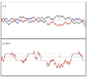
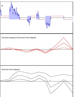
Figure 1: Plots of (a) two coupled Brownian motionsAandB, (b) the difference W =B−A=B(0)−A(0) +R(J−1)dA. The coupling controlJswitches be-tween values+1(“synchronous coupling”) and−1(“reflection coupling”). In the figure, switches to fixed periods ofJ = +1are triggered by successive crossings of±1byW.
B begun at different locationsA(0) andB(0): we shall suppose they are related by a stochastic integral B = B(0) +R JdA, where J is a piece-wise constant ±1-valued adapted random function. The coupling is defined by specifyingJ:
W = B−A = B(0)−A(0) +
Z
(J −1)dA , (1)
so thatW is constant on intervals whereJ = 1(holding intervals), and evolves as Brownian motion run at rate4on intervals whereJ =−1(intervals in whichW
is run at full rate). The coupling is illustrated in Figure 1.
So our coupling problem is reduced to a stochastic control problem: how should one choose adapted J so as to control W and V = V(0) + R Wdt to hit zero simultaneously?
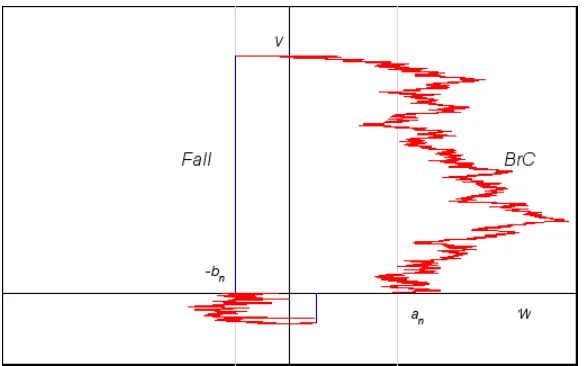
We start by noting that the trajectory (W, V) breaks up into half-cycles ac-cording to successive alternate visits to the positive and negative rays of the axis
V = 0. (We can assume V(0) = 0 without loss of generality; we can manipu-lateW andV to this end using an initial phase of controls!) We adopt a control strategy as follows: if the nth half-cycle begins at W =±a
n foran >0then we
compute a levelbndepending onan, withbn ≤ an ≤ κbnfor some fixed κ > 1,
and run this half-cycle of W at full rate (J = −1) until W hits∓bn or the
half-cycle ends. IfW hits∓bnbefore the end of the half-cycle then we start a holding
interval (J = 1) untilV hits zero, so concluding the half-cycle. Setan+1 to be the absolute value ofW at the end of the half-cycle. We will call the holding interval the Fall of the half-cycle and will refer to the initial component as the Brownian component or BrC. The construction is illustrated in Figure 2.
With appropriate choices for the an andbn, it can be shown that this control
forces(W, V)almost surely to converge to (0,0)in finite time. To see this, note the following. By the reflection principle applied to a Brownian motionB begun at0,
P[BrC duration ≥tn] ≤ P[2|B(tn)| ≤an+bn] ≤
an+bn
√
2πtn
. (2)
Simple dynamical arguments allow us to control the duration of the Fall:
Fall duration ≤ maxV during BrC
bn ≤
(BrC duration)×(maxW during BrC) bn
,
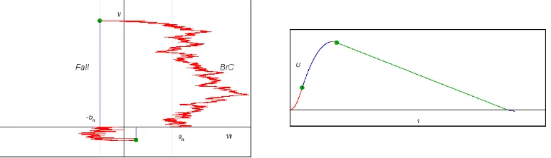
Figure 2: Illustration of two half-cycles for the casebn =an/2,κ = 2, labelling Fall and BrC for first half-cycle.
which we can combine with the following (forxn >0):
P[(maxW during BrC)≥xn] = P[2B+anhitsxnbefore −bn]
= an+bn an+bn+xn
. (4)
We now use a Borel-Cantelli argument to deduce that
Duration of half-cyclen ≤
µ
1 + xn bn
¶
tn (5)
for all sufficiently largen, so long as
X
n
an
√
tn
<∞, X
n
1 1 +xn/(2an)
<∞. (6)
(Bear in mind, we have stipulated thatbn ≤an ≤ κbn.) Now this convergence is
ensured by setting√tn=xn=ann1+α for someα >0, in which case we obtain
Duration of half-cyclen ≤
µ
1 + κxn an
¶
tn ≤
¡
1 +κn1+α¢a2
nn2+2α.
(7) If we arrange for an ≤ κ/n2+β then the sum of this overn converges, since we
Theorem 3.1 Suppose the evolution of(W,R Wdt)is divided into half-cycles as described above: if thenthhalf-cycle begins atW =±a
n, then it is run at full rate
tillW hits∓bnand then allowed to fall to the conclusion of the half-cycle. (The
fall phase is omitted if the half-cycle concludes beforeW hits∓bn.) Our control
consists of choosing the bn; so long as an/κ ≤ bn ≤ min{an,1/n2+β} for all
sufficiently largenfor some constantsκandβ >0, then(W,R Wdt)converges to(0,0)in finite time.
Remark 3.2 By definition of an we know an ≤ bn−1 ≤ 1/(n−1)2+β, so it is feasible to choosebnsuch thatan/κ≤bn ≤min{an,1/n2+β}for all largen.
Remark 3.3 Note thatanis determined by the location ofW at the end of
half-cyclen−1.
Remark 3.4 We can assume the initial conditionsW0 = 1,V0 = 0(otherwise we can run the diffusion at full rate tillV hits zero, as can be shown to happen almost surely, then re-scale accordingly). It then suffices to set bn = min{an,1/(n+
1)2+β}. However this is not the only option; for example Ben Arous et al. (1995)
usebn =an/2. Note, in either case we findan+1 ≤bn ≤an≤κbnforκ= 2.
3.2
Controlling two iterated integrals
Inspection of the above control strategy reveals some flexibility which was not exploited by Ben Arous et al. (1995); in the nth half-cycle there is a time T
n at
whichW first hits0, and we may then hold W = 0constant (by setting J = 1) and so delay for a timeCn, without altering either W orV =
R
Wdt. We may chooseCnas we wish without jeopardizing convergence of(W, V)to(0,0). This
flexibility allows us to consider controllingU =R R Wdsdtas follows: we hold atTnfor a duration long enough to forceU,V to have the same sign:
Cn = max
½
0,−
R R
Wdsdt
R
Wdt
¾
= max
½
0,−U V
¾
. (8)
The event[V(Tn) = 0]turns out to be of probability zero, since it can only happen
ifTnoccurs at the very start of the half-cycle, which in turn happens only ifW hits
zero exactly at the end of the previous half-cycle; that this is a null event will be a weak consequence of the lower bound at Inequality (16) below. The construction is illustrated in Figure 3.
Suppose an ≤ κ/n2+β as in the previous subsection. If we can show that
P
Figure 3: Two consecutive half-cycles for the case bn = an/2, together with a graph ofU against time. The disks signify time points at which there is an option to hold the diffusion to allowU to change sign if required.
withU hitting zero in infinitely many half-cycles accumulating atζand therefore also converging to0atζ. To fix notation, let us supposeW is positive at the start of the half-cycle in question. This ensures V > 0 at time Tn. So the issue at
hand is to control Cn by determining what makes −U = −
R R
Wdsdt large, and what makesV =R Wdtsmall at timeTn.
Consider−U at time Tn. At the start of the half-cycle we knowV = 0 and
W =an, so subsequent contributions make−U more negative and need not detain
us. At the start of the previous half-cycleU will be non-negative. Consequently an upper bound for−U at timeTnis given by
(Duration of half-cyclen−1)2
2 ×(−minimum value ofW over half-cyclen−1),
thus (given the work of§3.1) we may suppose that, eventually inn, at timeTnthe
quantity−U is bounded above by
1 2
µµ
1 + xn−1 bn−1
¶
tn−1
¶2
×xn−1 =
1 2
¡
1 +κ(n−1)1+α¢2a5n−1(n−1)5+5α.
(9) Now apply a Borel-Cantelli argument and the reflection principle to show that eventually innthe Brownian component takes time at leasta2n/(4n2+2α)in
travel-ling fromantoan/2. We deduce almost surely for all sufficiently largen at time
Tnit must be the case thatV =
R
Wdtexceeds
(an/2)×time to move fromantoan/2 ≥
a3
n
ThusCnis bounded above, eventually inn, by
This leads to the crux of the argument; we need an eventual upper bound on the ratioan−1/an.
First note that the lower bound of Inequality (10), applied to the(n−1)stcycle, shows that eventually inn
−
So it suffices to obtain a suitable lower bound onan, the value ofW at the end of
half-cyclen−1, in terms of−RTn
−1Wdtand holding eventually inn. Moreover
we may ignore the Fall component of half-cyclen−1so long as the lower bound is smaller thanbn−1, and treatW over the whole of this half-cycle as a Brownian motion of rate4.
We now introduce a discontinuous time-change based on the continuous (but non-monotonic) additive functionalV(t) = R Wds: condition onRTn Consequently, on time intervals throughout whichZ >e 0,
dZe(u) = p2 e
Z
dBe whenZ >e 0 (13)
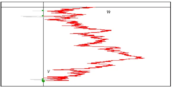
for a new standard Brownian motionBe. The time-changed processZeis illustrated in Figure 4. Note thatZemust be non-negative.
A nonlinear transformation of scale Z = Ze3/2/3 produces a Bessel(4 3) pro-cessZ in time intervals throughout whichZe(equivalentlyZ) is positive: by Itˆo’s formula the stochastic differential equation
Figure 4: Discontinuous time-change for W based on V = R Wdt. The effect of the time-change is to delete the loops extending into W > 0, and to continue deletion tillV = R Wdtre-attains its minimum, thus generating discontinuities (some of which are indicated in the figure by small dots on the V-axis) in the time-changed processZ, which follows the red /dark trajectory.e
holds in intervals for whichZ >0.
Now observe that the zero-set {u : Z(u) = 0} is almost surely a null-set. For certainly the Brownian zero-set {t : W(t) = 0} is almost surely null, and {V(t) : W(t) = 0} is then almost surely null by Sard’s lemma, sinceV is aC1 function with derivativeW (indeed this is an easy exercise in this simple context). But{u:Z(u) = 0}={u:Ze(u) = 0}is a subset of{V(t) :W(t) = 0}.
Because{u:Z(u) = 0}is almost surely a null-set, it follows that the stochas-tic integral
B(u) =
Z u
0 I
[Z >0]dBe (14)
(using Equation (13) to construct Be when Z > 0) defines a Brownian motion. Furthermore we can apply limiting arguments to write
Z = B+ 1 6
Z
I[Z >0] 1
Z du+H (15)
whereHis the non-decreasing pure jump process
H(u) = X
v≤u
1
3(W(σ(u))−W(σ(u−)))
3/2
,
Using the theory of the Skorokhod construction (El Karoui and Chaleyat-Maurel 1978), we now derive the comparison
Z ≥ B +L
whereLis local time ofB at0, so thatB +Lis reflected Brownian motion. (H
is discontinuous, but the argument of the Skorokhod construction applies so long asHis non-decreasing.) Consequently
P
·
1 3Ze
3/2(u
n−1)≥x
¸
≤ P[B(un−1)≥x]
and so we can deduce from a Borel-Cantelli argument and the lower bound of Inequality (12) that the following holds eventually inn:
an ≥
Ã
|RTn
−1Wdt
|
(n−1)2+2α
!1/3
≥ an−1
µ
1 8(n−1)4+4α
¶1/3
(16)
forα >0. Thus eventually inn
Cn ≤ 32
¡
1 + (n−1)1+α¢2(n−1)9+9αn2+2α×a2n−1
and so we can arrange for PnCn < ∞ so long as we choose an ≤ 1/n7+β for
β >0.
We state this as a theorem:
Theorem 3.5 The modified strategy described at the head of this subsection (hold at each Tn till
R R
Wdsdt is zero or has the same sign as R Wdt) produces convergence of
(W,
Z
Wdt,
Z Z
Wdsdt)
to(0,0,0)in finite time so long as the conditions of Theorem 3.1 are augmented by the following: half-cycle n begins atW = ±an foran ≤ 1/n7+β for β > 0
and for all sufficiently largen. (This can be arranged by choosingbnin the range
an/κ≤bn ≤min{an,1/n7+β}for constantsκandβ >0.)
Remark 3.6 The choicebn=an/2of Ben Arous et al. (1995) will suffice.
square of a standard normal random variable. This argument permits replacement of Equation (10) by
Z Tn
Wdt ≥ constant×a3n√1 n.
Remark 3.8 The elementary comparison approach above can of course be re-placed by arguments employing the exact computations of McKean (1963).
Remark 3.9 The method described here (control coupling of higher-order iterated integrals by judicious waits atW = 0) appears to deliver effective control of just one higher-order iterated integral in addition to W, V = R Wdt. Attempts to control more than one higher-order iterated integral seem to lead to problems of propagation of over-correction from one half-cycle to the next. We therefore turn to a rather different, less explicit, approach in the remainder of the paper.
4
Reduction to non-iterated time integrals
Before considering the problem of coupling more than two iterated time inte-grals, we first reformulate the coupling problem in terms of integrals of the form
R tm
m!B(t)dtrather than the less amenable iterated time integrals of above. We be-gin with some notation. Suppose W is defined as the difference between two co-adapted coupled Brownian motions, as in§3.1. Then we setW =W(0) =B−A and define the firstN iterated time integrals inductively by
W(1) = W(1)(0) +
Z
W(0)dt ,
W(2) = W(2)(0) +
Z
W(1)dt ,
. . .
W(N) = W(N)(0) +
Z
W(N)dt . (17)
conditions all vanish, then we find by exchange of integrals that
Binomial expansion leads to the following:
Lemma 4.1 SupposeW(0)(0) =W(1)(0) = W(2)(0) =. . .=W(N)(0) = 0, and
J is a given adapted control, andζis a given stopping time. Then
W(0)(ζ) = 0, W(1)(ζ) = 0, W(2)(ζ) = 0, . . . , W(N)(ζ) = 0
If the iterated time integrals have non-zero initial values then we can reduce to the case of zero initial values by supposing W is deterministically extended backwards in time to time −1, with corresponding generalization of Equation (17). By a simple argument using orthogonal Legendre polynomialsPnon[−1,1],
Expanding the Legendre polynomials and adapting the argument leading to Lemma 4.1, we can find a1, . . . , aN in terms of b0, b1, . . . , bN−1 by solving a triangular linear system of equations. Finally,bN andbN+1may be fixed by the requirement that W(0) = a0 = PNn=0+1bnPn(1) and 0 = W(−1) = PNn=0+1bnPn(0) (note
that Legendre polynomials do not vanish at their end-points, and are odd or even functions according to whether their order is odd or even!).
This allows us to use Lemma 4.1 to deduce the required reduction:
Lemma 4.2 It is possible to use adapted controlsJ to ensure
W(0)(ζ) = 0, W(1)(ζ) = 0, W(2)(ζ) = 0, . . . , W(N)(ζ) = 0
at some stopping timeζ (depending on initial valuesW(n)(0)) if and only if it is also possible to use adapted controls to ensure
W(ζ) = 0,
b0+
Z ζ
0
W(t)dt = 0, b1 +
Z ζ
0
tW(t)dt = 0,
. . . , bN−1+
Z ζ
0
tN−1
(N −1)!W(t)dt = 0.
(Here the constants bn depend on the initial conditions W(n)(0) for the iterated
integrals).
For we may extend back over[−1,0], condition on achieving the desired values {W(n)(0) :n = 0, . . . , N}, and work with controlsJ which act only for positive time.
5
Coupling finitely many iterated integrals
To motivate the control strategy required to couple more than two iterated inte-grals, we consider a discrete analogue to our problem which is in fact a limiting case.
Suppose we choose only to switch between J = ±1 at instants when W
R tm
m!dW: if we holdJ = +1 at successive levels±1, beginning at+1, making switches from ±1 to ∓1 at times 0 = T0 < T1 < . . . < Tr, then (under the
instantaneous switching approximation)
Z Tr
0
tm
m!dW =
r−1
X
k=0
(−1)kT
m+1
k+1 −Tkm+1
(m+ 1)! . (18)
In §5.1 below we show that particular patterns of switching times produces zero effect on integrals up to a fixed order, at least for the discrete analogue. This permits us to eliminate a whole finite sequence of the integrals. (Of course in practice, because switching is not instantaneous, the use of such patterns creates further contributions to the integrals which then must be dealt with in turn!)
It is algebraically convenient to formulate the required patterns using a se-quenceS0,S1, . . .S2N
−1of values of±1defined recursively in a manner reminis-cent of the theory of experimental design. We set
S0 = +1,
(S2n, S2n+1, . . . , S
2n+1
−1) = −(S0, S1, . . . , S2n−1). (19)
Here is the pattern formed by the first sixteenSnvalues:
+ - - + - + + - - + + - + - - +
We will be considering perturbations and re-scalings of the deterministic control which applies control J = −1 throughout the time interval [m, m + 1) till a switch has occurred to level Sm, and then applies J = 1 for the remainder of
the time interval. The discrete analogue can be viewed as a limiting case under homogeneous (not Brownian!) scaling of space and time. See Figure 5 for an illustration.
5.1
Algebraic properties of the sign sequence
We now prove some simple properties of the sign sequenceS0,S1, . . .S2N
−1.
Lemma 5.1 Ifb(r)is the number of positive bits in the binary expansion ofrthen
Proof:
Sinceb(0) = 0this holds forS0 = 1. The recursive definition (19) shows that if the lemma holds for the first2nentries in the sequence ofS
nthen it will also hold
for the next2nentries. The result follows by induction.
¤
The proofs of the next three corollaries are immediate from the recursive def-inition of theSm’s.
Corollary 5.2
S2ℓj+a = SjSa whena= 0,1, . . . ,2ℓ−1.
Corollary 5.3
S2m+1 = −S2m
Notice the analogue of Corollary 5.3 does not hold betweenS2m+2andS2m+1!
Corollary 5.4
2n
−1
X
m=0
Sm = 0 ifn≥1,
= 1 ifn= 0.
These results imply the vanishing of certain sums of low-order powers:
Lemma 5.5
2N
−1
X
m=0
(m+ 1)k
k! Sm = 0 ifk < N ,
= (−1)N2N(N−1)/2 ifk =N . (20)
Proof:
Use induction on the level k. If k = 0 then Equation (20) follows from the expression for P2
N
−1
m=0 Sm in Corollary 5.4. Hence Equation (20) holds at level
Suppose Equation (20) holds for all levels below levelkand supposek < N. Using the recursive construction (19),
2N
using the binomial expansion and cancelling the (m+ 1)k terms. Now we can
apply the inductive hypothesis to dispose of terms involving(m+1)k−uforu >1:
2N
Thus Equation (20) follows by applying the inductive hypothesis to the right-hand
side. ¤
Remark 5.6 An alternative approach uses generating functions, applying the re-cursive construction of Equation (19) to show
∞
We can now compute the discrete analogue ofR2
N
0
tm
m!W(t)dt under the spe-cial control which arranges instantaneous switching to levelSmat timem.
Theorem 5.7 For allk < N
¤
Note that Equation (21) forS0, S1, . . . , S2N
−1 is equivalent to Equation (18) with appropriate definitions of the switching timesT0, T1, . . . ,Tr. We now
intro-duce notation for these deterministic times, as they will be basic to our coupling construction.
Definition 5.8 Define switching timesTe1, . . . , Ter(N) to be the times m at which
Sm−1 =±1switches toSm =∓1, and setTe0 = 0.
Corollary 5.9 By induction onN ≥1, sincer(N+ 1) ≥2r(N),
N ≤ r(N) ≤ 2N −1.
5.2
Application to the coupling problem
We can now summarize our control strategy for successful coupling. By global analysis (specifically, the inverse function theorem), as long as initial conditions for integrals of order up to R tN−1
(N−1)!Bdt are sufficiently small we can obtain a perturbationT0
0 = 2N < T10 < . . . < Tr0(N) of the switching timesTe1, . . . ,Ter(N) (Definition 5.8) which will dispose of these initial conditions by time2N. (As will
become apparent, scaling arguments can be deployed to deal with larger initial conditions.)
Since the coupled Brownian motions cannot actually produce instantaneous transitions between ±1, the switching activity will have introduced further non-zero contributions to the integrals by time2N. So long as these contributions are
in turn sufficiently small, we can dispose of them in turn by administering a new control based on switching times T1
0 = 2N < T11 < . . . < Tr1(N) which form a small perturbation of the scaled control obtained fromTe1, . . . ,Ter(N)by re-scaling both space and time homogeneously by a factor 1/2(not by Brownian scaling!) and shifting forwards in time by 2N. Thus switching now occurs between levels ±1/2. A key reason for the success of the coupling is that in terms of Brown-ian scaling there is now twice as much effective time in which to carry out each switch! This means that the probability of all switches completing within their assigned times will increase rapidly to1.
bound on the probability of this infinite sequence completing before a finite time: and moreover the size of the integrals decreasing to zero.
If this fails (because at some stage no small enough perturbation is available, or because a switch fails to complete before its successor is due) then we simply restart the procedure, scaling time to ensure existence of the perturbation re-quired initially. Continuing in this manner allows us to deduce that almost surely coupling is eventually successful.
All depends on analyzing the behaviour of perturbations of deterministic con-trols of the form of Definition 5.8. Consider the map whose coordinates corre-spond to analogues of time integrals of order less thanN:
F(t0;t, u) = F(t0;t1, . . . , tN, uN+1, . . . , ur(N)) = (F0, . . . , FN−1) (22)
This is proportional to a Vandermonde determinant and in fact evaluates to
2N(−1)N
1·1·2!·. . .·(N −1)!
Y
1≤i<j≤N
which is non-zero so long as the ti’s are distinct. This and the inverse function
theorem allows us to assert the following fact:
Lemma 5.10 The polynomial (hence smooth) map
t = (t1, . . . , tN) 7→ F(0;t,TeN+1, . . . ,Ter(N))
is invertible in a neighbourhood of the initial sequence of switching times Te0,
e
T1, . . . ,TeN corresponding to switching between levelsSm, . . . at timesm, . . . . In
particular there isκ >0andε′ >0
such that for allε < ε′
, if|W(m+1)(0)|< εfor
m = 0,1, . . . ,N −1, then there is aκε-perturbation(t1, . . . , tN)of(Te1, . . .TeN)
with 0 < t1 < . . . < tN < TeN+1 (hence generating a valid switching strategy) which is such that
Fm(0;t1, . . . , tN,TeN+1, . . . ,Ter(N)) = −W(m+1)(0)
form= 0,1, . . . ,N −1.
Note further that from Equation (22) and the binomial theorem we have a translation symmetry:
Lemma 5.11
Fm(t0+s;t+s, u+s) =
m
X
u=0
sm−u
(m−u)!Fu(t0;t, u)
while Equation (22) directly yields a scaling property:
Lemma 5.12
Fm(λt0;λt, λu) = λm+1Fm(t0;t, u).
We need just one more lemma, concerning the behaviour of Brownian motion, before we can state and prove the main coupling result for this section.
Lemma 5.13 Consider a Brownian motionBstarted at0and run till it hits level −3/2at timeS. For fixed constantsK1,K2
X
n
P
"
S > K1(1 +n)2+2αor sup [0,S]
B > K2(1 +n)2+2α
#
Proof:
This follows easily from the reflection principle and elementary Gaussian integral estimates:
P
"
S > (1 +n)2+2αor sup
[0,S]
B >(1 +n)2+2α
#
≤ 1−2P
·
B(1 +n)2+2α <−3 2
¸
+ 2P£B((1 +n)2+2α)>(1 +n)2+2α¤
≤ √2
2π
Z 3
2(1+n)1+α)
− 3
2(1+n)1+α)
e−u2/2du+√2
2π
Z ∞
(1+n)1+α
e−u2/2du
≤ √5
2π 1 (1 +n)1+α .
¤
Theorem 5.14 There is a successful co-adapted coupling for Brownian motion and its firstN iterated time integrals.
Proof:
By the work of§4 this is reduced this to the problem of finding an adapted control
J = ±1 which delivers W such that at a particular stopping time ζ we have
W(ζ) = W(0)(ζ) = 0andW(m+1)(0) +Rζ 0
tm
m!W(t)dt = 0form = 0, 1, . . . ,
N −1. Without loss of generality we assume W(0) = 2(for otherwise we can run the controlJ =−1till this occurs!).
Using Lemma 5.10 and Lemma 5.12, for fixedε > 0we can chooseC large enough to solve for(t0
1, . . . , t0N)with|t0k−Tek|< εin
Fm(0;Ct01, . . . , Ct0N, CTeN+1, . . . , CTer(N)) = −W(m+1)(0) (25)
for m = 0, . . . , N − 1: carry out this switching strategy over the time period
[0,2NC)to eliminate the initial conditions.
Stepk: At timeTk
0 = (2−21−k)2NC, use Lemmas 5.10, 5.11, and 5.12 to determine the solution(tk
1, . . . , tkN)of
(taking into account that previous steps will have eliminatedRT
k or equivalently (Lemmas 5.11, 5.12)
Fm(0;tk1, . . . , tkN,TeN+1, . . . ,Ter(N)) Apply the switching strategy determined byTk
0,T1k, . . . ,Trk(N)over the time interval[Tk
0, T0k+1).
The algorithm can fail at this step if either the integralsRT
k
0 0
tm
m!W(t)dtare too large, or one of the2N switches fails to complete in the interval allotted to it. The
estimate of Lemma 5.13 allows us to obtain bounds on (a) the probability of large
size of the integralsRT
k and (b) the probability that a switch begun at Tk
r−1 fails to complete by time the next switchTk
r is due to start.
Set Z−1
α = supk=0,1,...(1 + k)1+α2−k/2, for some fixed α > 1, and recall
from Lemma 5.10 that ε > 0 is the bound on initial conditions required if κε -perturbation switching controls are guaranteed to exist. LetDk be the event that
form= 0, . . . ,N −1, and also and so (bearing in mind the effects of the switching strategy) Dk holds only if
W(Tk
ensures we will be able to determine the solution(tk
1, . . . , tkN)in Equation (25). crossing may be replaced by a down-crossing from2−kto−2−k, or an up-crossing
from −2−k to 2−k (but this does not decrease the probability of the event
con-cerned!).
By Brownian scaling any one such event has probability bounded above by the probability of the following event:
sup
andW makes an down-crossing from 2
−(k−1)/2
can use the Markov property and the density of Brownian paths to deduce there is a positive chancep >0thatTkFkoccurs. If this happens then coupling succeeds
6
Impossibility of coupling all iterated integrals
Is it possible to arrange successful coupling for all iterated integrals at a single stopping timeζusing some adapted controlJ?
Summation of the coupling statements produces a statement about Laplace transforms of the path, which allows us to demonstrate that coupling of all iterated integrals is possible only in trivial cases.
Theorem 6.1 Suppose that the initial conditions for the iterated stochastic inte-grals are feasible, in the sense that they could have been produced by integration of a continuous path starting at some previous time (without loss of generality, time−1). Consider an adapted controlJ producing coupling for all iterated in-tegrals at a stopping timeζ. This can be produced only ifW =B−Ais actually identically zero over[0, ζ].
Proof:
Suppose the Brownian paths and all iterated integrals couple atζ, soW(n)(ζ) = 0 for alln. We show that in this caseW ≡0must hold over the interval[0, ζ].
By hypothesis, we may convert into statements about integrals over [−1, ζ]
(with a suitable extension ofW) using powers oft. We can write
∞
X
n=0
βn
Z ζ
−1
tn
n!W(t)dt = 0.
The continuous pathW is bounded over[−1, ζ], so the sum on the left-hand-side converges and moreover we can exchange integral and summation to obtain
Z ζ
−1
exp(βt)W(t)dt = 0
for allβ. By uniqueness of the Laplace transform, this holds only ifW ≡0over
the interval[0, ζ]as required. ¤
Remark 6.2 This argument is essentially non-stochastic, based only on the con-tinuity of the path which is the difference of the two coupled processes, and so holds for any coupling, whether co-adapted or not.
7
Conclusion
We conclude by noting that the successful coupling strategies of §3 and §5 are both in essence very simple, involving switching between synchronous (J = 1) and mirror (J = −1) coupling. It would be interesting to construct a successful coupling strategy which optimized, for example, a specific exponential moment of the coupling time; one expects there would be a whole family of such couplings parametrized by the coefficient in the exponential moment, and that the coupling strategies themselves would have some kind of geometric flavour.
The results of this paper can be viewed as introducing a new notion to coupling theory: that of an “exotic coupling”, a co-adapted coupling for a diffusion (in this case real Brownian motion) which successfully couples not only the diffusion itself but also a number of path functionals of the diffusion. It is striking that exotic coupling is feasible at all; the method of proof for the general case (§5) is very suggestive for how to address more general situations. Ben Arous et al. (1995) also showed the existence of an exotic coupling for planar Brownian motion using the path functional given by the L´evy stochastic area, and it would be interesting to see how far the Ben Arous et al. (1995) result could be extended to higher dimensional Brownian motion; this would be a useful next step towards the natural bold conjecture which we now present:
Conjecture 7.1 Hypoelliptic diffusions with smooth coefficients can be coupled co-adaptively with positive chance of success from any two starting points.
It would of course be of great interest to obtain specific applications of these couplings, perhaps for example in Coupling from the Past constructions.
Finally we remark that Price (1996) gives some results concerning exotic cou-pling using single functionals of the formR f(t)Bdt.
References
Aldous, D. J. and H. Thorisson (1993). Shift-coupling.
Ben Arous, G., M. Cranston, and W. S. Kendall (1995). Coupling constructions for hypoelliptic diffusions: Two examples. In M. Cranston and M. Pinsky (Eds.),
Burdzy, K. and W. S. Kendall (2000, May). Efficient Markovian couplings: examples and counterexamples.
Chen, X. and W. V. Li (2003). Quadratic functionals and small ball probabilities for the m-fold integrated Brownian motion.
Corwin, L. J. and F. P. Greenleaf (1990). Representations of nilpotent Lie groups and
their applications. Part I, Volume 18 of Cambridge Studies in Advanced Mathe-matics. Cambridge:
Cranston, M. and F.-Y. Wang (2000). A condition for the equivalence of coupling and shift coupling.
El Karoui, N. and M. Chaleyat-Maurel (1978). Un probl`eme de r´eflexion et ses ap-plications au temps local et aux ´equations diff´erentielles stochastiques surR, cas continu. In J. Azema and M. Yor (Eds.), Temps Locaux, Volume 52-53, pp. 117– 144.
Goldstein, S. (1978 – 1979). Maximal coupling. Zeitschrift f¨ur
Wahrscheinlichkeits-theorie und Verve Gebiete 46(2), 193–204.
Griffeath, D. (1974 / 1975). A maximal coupling for Markov chains. Z.
Wahrschein-lichkeitstheorie und Verw. Gebiete 31, 95–106.
Groeneboom, P., G. Jongbloed, and J. A. Wellner (1999). Integrated Brownian motion, conditioned to be positive.
Hayes, T. P. and E. Vigoda (2003). A non-Markovian coloring for randomly sampling colorings. Technical report, Dept. Computer Science, University of Chicago. To appear in FOCS 2003. Preliminary version available.
Jerrum, M. (2003). Counting, sampling and integrating: algorithms and complexity. Lectures in Mathematics ETH Z¨urich. Basel: Birkh¨auser Verlag.
Ka˘ımanovich, V. A. (1986). Brownian motion and harmonic functions on covering manifolds. An entropic approach. Dokl. Akad. Nauk SSSR 288(5), 1045–1049.
Kendall, W. S. (1986). Stochastic differential geometry, a coupling property, and har-monic maps. 554–566.
Kendall, W. S. (1994). Probability, convexity, and harmonic maps II: Smoothness via probabilistic gradient inequalities.
Khoshnevisan, D. and Z. Shi (1998). Chung’s law for integrated Brownian motion.
Lachal, A. (1997). Local asymptotic classes for the successive primitives of Brownian motion.
Leeb, B. (1993). Harmonic functions along Brownian balls and the Liouville property for solvable Lie groups. Math. Ann. 296(4), 577–584.
Lyons, T. J. and D. Sullivan (1984). Function theory, random paths and covering spaces. J. Differential Geom. 19(2), 299–323.
McKean, H. (1963). A winding problem for a stochastic resonator driven by a white noise. Journal of Mathematics of Kyoto University 2, 227–235.
Price, C. J. (1996). Zeros of Brownian polynomials and Coupling of Brownian areas. Ph. D. thesis, Department of Statistics, University of Warwick.
Propp, J. G. and D. B. Wilson (1996). Exact sampling with coupled Markov chains and applications to statistical mechanics. 223–252.