ELECTRONIC COMMUNICATIONS in PROBABILITY
SCALING LIMIT OF THE PRUDENT WALK
VINCENT BEFFARA
UMPA – ENS Lyon, 46 Allée d’Italie, 69364 Lyon Cedex 07, France
email: [email protected]
SACHA FRIEDLI
Departamento de Matemática, UFMG-ICEX C.P. 702, Belo Horizonte, 30123-970 MG, Brasil
email: [email protected]
YVAN VELENIK
Section de Mathématiques, Université de Genève, 2-4 rue du Lièvre, 1211 Genève 4, Suisse
email: [email protected]
SubmittedJuly 2, 2009, accepted in final formFebruary 9, 2010 AMS 2000 Subject classification: 60F17, 60G50, 60G52
Keywords: prudent self-avoiding walk, brownian motion, scaling limit, ballistic behaviour, ageing
Abstract
We describe the scaling limit of the nearest neighbour prudent walk onZ2, which performs steps uniformly in directions in which it does not see sites already visited. We show that the scaling limit is given by the process Zu=
R3u/7
0 σ11{W(s)≥0}~e1+σ21{W(s)<0}~e2
ds,u∈[0, 1], whereW is the one-dimensional Brownian motion andσ1,σ2two random signs. In particular, the asymptotic speed of the walk is well-defined in the L1-norm and equals 37.
1
Introduction and description of results
The prudent walk was introduced more than 20 years ago, under the name self-directed walk
in [11, 12] andoutwardly directed self-avoiding walk in [9], as a particularly tractable variant of the self-avoiding walk. Interest in this model has known a vigorous renewal in recent years, mostly in the combinatorics community[5, 6, 4, 3, 10, 2]. The latter works are concerned with a variant of the original model, more natural from the combinatorial point of view, obtained by considering the uniform probability measure on all allowed paths of given length; we’ll refer to it as the uniform prudent walk. In the present work, we consider the original (kinetic) model and describe its scaling limit in details.
Let~e1= (1, 0),~e2= (0, 1)denote the canonical basis ofZ2. Let us describe the construction of
the process associated to the prudent random walkγ·. We first setγ0:= (0, 0). Assume that we have already constructed1γ[0,t], then the distribution ofγt+1is obtained as follows. We say that the direction~e∈ {±~e1,±~e2}is allowed if and only if{γt+k~e,k>0} ∩γ[0,t]=∅; in other words,
1For any discrete- or continuous-time processY
t, we denote byY[0,t]:={Ys}0≤s≤t.
allowed directions are those towards which there are no sites that have already been visited.γt+1
is chosen uniformly among the neighbours ofγt lying in an allowed direction. Observe that there are always at least two allowed directions.
There has been considerable interest in such non-Markovian processes recently. Among the moti-vations are the necessity of developing specific methods to analyse these processes, and the fact that they sometimes present rather unusual properties. From this point of view, the prudent walk is quite interesting. On the one hand, it is sufficiently simple that a lot of information can be extracted, on the other its scaling limit possesses some remarkable features.
Our main result is the following, which describes the scaling limit (in a topology stronger than weak convergence) of the prudent walk.
Theorem 1.1. On a suitably enlarged probability space, we can construct the prudent walk γ·, a Brownian motion W·and a pair of±1-valued random variablesσ1,σ2such that
lim
t→∞P 0≤sups≤t
1
tγs−Z σ1,σ2
s/t
2> ε
=0,
where, for u∈[0, 1],
Zσ1,σ2
u :=
Z3u/7
0
σ11{W(s)≥0}~e1+σ21{W(s)<0}~e2
ds. (1)
The Brownian motion W·and the two random signsσ1,σ2are independent of each other, and P(σ1= s,σ2=s′) =1/4, for s,s′∈ {−1, 1}.
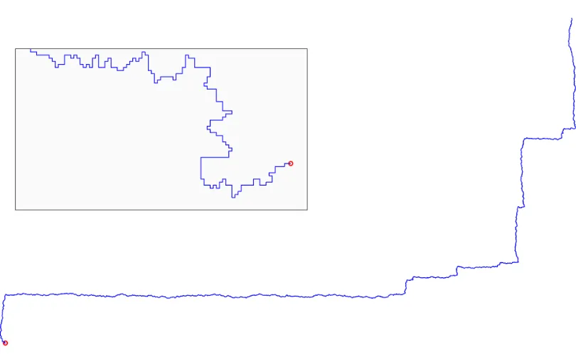
A typical trajectory ofγ·is depicted in Fig. 1. Let us briefly discuss some of the consequences of Theorem 1.1. To simplify the exposition, we assume thatσ1=σ2=1 (with no loss of generality, given the obvious symmetries of the prudent walk).
• SincekZu1,1k1 = 3u/7, the asymptotic speed of the prudent walk converges to 3/7 in L 1
-norm in probability. Note that there is no asymptotic speed in theL2-norm. Actually, using arguments very similar to those of Section 4, one can prove that the speed converges almost surely to 3/7.
• The angleαubetweenZ1,1
u and~e1is random, which means that the prudent walk undergoes
macroscopic fluctuations in direction, even though it is ballistic. The distribution ofαucan easily be determined, using the arcsine law for Brownian motion:
P(αu≤x) =P(tanαu≤tanx) =P θ
+(W [0,u])
u ≥
1 1+tanx
= 2
πarctan p
tanx, whereθ+(W[0,u])is the time spent byW[0,u]above 0.
• The presence of heavy-tailed random variables (the length of the Brownian excursions) in the limiting process Z·1,1 allows the construction of various natural observables displaying ageing. For example, its first component.
Figure 1: The first 50000 steps of a prudent walk. The inset is a blow-up of the first few hundred steps near the origin.
a simpler variant of the latter (similar to our corner model, see below) that the scaling limit is a straight line along the diagonal, with a speed inL1-norm approximately given by 0.63. We expect
the same to be true for the real uniform prudent walk.
We also observe that our scaling limit is radically different from what is observed for similar contin-uous random walks that avoid their convex hull, which again are ballistic but, at the macroscopic scale, move along a (random) straight line ([13],[1]).
Acknowledgements: We are grateful to Bálint Tóth for suggesting the representation (1) for the scaling limit, substantially simpler than the one we originally used. We also thank two anonymous referees for their careful reading. SF was partially supported by CNPq (bolsa de produtividade). Support by a Fonds National Suisse grant is also gratefully acknowledged.
2
Excursions
We split the trajectory of the prudent walk into a sequence of excursions. To a path γ[0,t], we associate the bounding rectangleRt⊂Z2with lower left corner(xmin,ymin), and upper right corner (xmax,ymax). Here,xmin=minAt, ymin=minBt,xmax=maxAt, ymax=maxBt, where
At :=
¦
x∈Z:∃y∈Z,(x,y)∈γ[0,t]©,Bt:=
¦
say that the path visits a corner at times∈ {0, . . . ,t}ifγscoincides with one of the four corners of
Rs.
Without loss of generality, we assume that the first step of the path is in the direction~e1, i.e.,
γ1=~e1, and define the following sequence of random times: T0:=0 ,
U0:=inft>0 :Ht>1 −1 , and fork≥0,
Tk+1=inf
t>Uk :Wt >Wt−1 −1 , Uk+1=inft>Tk+1 :Ht >Ht−1 −1 .
During the time interval(Tk,Uk], the walk makes an excursion, denotedEkv, along one of the vertical sides ofRt. During the time interval(Uk,Tk+1], the walk makes an excursion, denotedEkh, along one of the horizontal sides ofRt. Two relevant quantities are the horizontal displacement ofEv
k:Xk:=WTk+1− WTk, and the vertical displacement ofE
h
k:Yk:=HTk+1− HTk. Observe that by
construction,Xk≥1 andYk≥1.
R
Tk+1
T
k0
R
TkU
kT
k+1Figure 2: The excursions and their associated times.
2.1
The effective random walk for the excursions
As Figure 2 suggests, the study of excursions along the sides of the rectangle can be reduced to that of the excursions of an effective one-dimensional random walk, with geometric increments.
Letξ1,ξ2, . . . be an i.i.d. sequence,ξi∈Z, withP(ξi=k) = 1 3(
1 2)|
k|. LetS
0=0,Sn=ξ1+· · ·+ξn. We callSnthe effective random walk. LetηLbe the first exit time ofSnfrom the interval[0,L−1]:
ηL:=inf{n>0 :Sn6∈[0,L−1]}. The following lemma will be used repeatedly in the paper.
Lemma 2.1. For all k≥0, m≥1,
P(Xk=m|γ[0,Tk]) =P(ηH
Tk =m), (2)
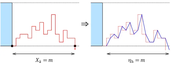
Proof. We show (2). Assume that the walk is at the lower right corner of the rectangle at time
Tk. On{Xk=m} ∩ {HTk=h}, the excursionEv
kcan be decomposed into(α1, . . . ,αm−1,β), where
eachαi is an elementary increment made of a vertical segment of lengthli∈[−h+1,h−1]∩Z
and of a horizontal segment of length 1 pointing to the right, andβ is a purely vertical segment of lengthl∈[−h,+h]∩Z, which ensures that the excursion reaches either the top or the bottom of the rectangle by timem(see Figure 3). We thus have
P(Xk=m|γ[0,Tk]) =
X
(α1,...,αm−1,β)
p(α1). . .p(αm−1)p(β),
where the sum is over all possible sets of such elementary increments, andp(αi) = 1 3(
1 2)|
li|,p(β) =
1 3(
1 2)
|l|−1. Therefore, in terms of the effective random walk with incrementsξ
i,
p(α1). . .p(αm−1) =P(ξ1=l1, . . . ,ξm−1=lm−1).
Moreover, ifl<0 (as on Figure 3), then
p(β) =1 3(
1 2)
|l|=1 3
X
j≥|l|+1 (1
2)
j
≡P(Sm<0|Sm−1=|l|).
Similarly, ifl≥0
p(β) =P(Sm≥h|Sm−1=h−l−1). This shows that
P(Xk=m|γ[0,Tk]) =P(S1∈[0,h−1], . . . ,Sm−1∈[0,h−1],Sm6∈[0,h−1]), which is (2).
⇒
Xk=m ηh=m
Figure 3: The decomposition of the excursionEv
k. The full segments on the right image represent the increments of the effective random walkSn. Observe thatSnstarts at γTk+1, and that it exits [0,h−1]at timemby jumping to any point on the negative axis.
3
Crossings and visits to the corners
possibility of winding around the origin an infinite number of times, and will allow in the sequel to restrict the study of the prudent walker to a single corner of the rectangle.
LetAk denote the event in which thekth excursion crosses at least one side ofRTk, that is if the
walk is at a bottom (resp. top) corner of the box at timeTkand at a top (resp. bottom) corner of the box at timeUk, or if it is at a right (resp. left) corner of the box at timeUkand at a left (resp. right) corner of the box at timeTk+1.
Proposition 3.1. There exists a constant c1>0such that P(Ak)≤ c1
k4/3 (4)
for all large enough k. In particular, P(lim supkAk) =0, and a.s. exactly one of the corners is visited
infinitely many times.
For k large, the bounding rectangle has long sides, which makes crossing unlikely. As is well known from the gambler’s ruin estimate for the simple symmetric random walk, the probability of first leaving an interval of length L at the opposite end is of orderL−1. To obtain (4), it will therefore be sufficient to show that the sides of the rectangle at the kth visit to a corner grow superlinearly ink.
Before this, we give a preliminary result for the effective random walkSn starting at 0. Let as beforeηL denote the first exit time of Sn from the interval[0,L−1]. We will also useη∞ :=
inf{n>0 :Sn<0}.
Lemma 3.1. There exists a constant c2>0such that for all L≥1, P(ηL≥n)≥pc2
n for all integer n≤c2L
4/3. (5)
Proof. Defineη→
L :=inf{n>0 :Sn≥L−1}, so that
P(ηL≥n) =P(η∞≥n,η→
L ≥n)
=P(η∞≥n)−P(η→L <n,η∞≥n)
≥P(η∞≥n)−P(η→
L <n). By the gambler’s ruin estimate of Theorem 5.1.7. in[8],
P(η∞≥n)≥pc3
n (6)
for some constantc3>0. On the other hand,
P(η→L <n)≤P(max
1≤j≤n|Sj| ≥L)≤
E[|Sn|2] L2 =
2n L2
The second inequality follows from the Doob-Kolmogorov Inequality.
As a consequence, we can show that by thekth visit to the corner, the sides of the rectangle have grown by at leastk4/3. A refinement of the method below actually shows thatWTk andHTk grow
Lemma 3.2. There exist positive constants c4and c5such that
P(WTk<c5k4/3)≤exp −c4k1/3, (7)
P(HTk<c5k4/3)≤exp −c4k1/3
. (8)
Proof. Letm=⌊k/2⌋. SinceXi≥1 andYi≥1 for all i, we have thatHTj ≥m,WTj ≥m, for all
j≥m. We consider the width of the rectangle at timeTk. LetIjdenote the indicator of the event
{Xj≥c2m4/3}. We have, for all j≥m,
P(Ij=1|γ[0,Tj]) =P(Ij=1| HTj)
=P(ηH
T j ≥c2m
4/3)
≥P(ηm≥c2m4/3)
by (5)≥c−23/2m−2/3≡p.
Therefore, the Ijs can be coupled to Bernoulli variables of parameterp. SinceWTk =
Pk−1
j=0Xj≥
c2m4/3
Pk−1
j=mIj, we get
P(WTk<2−4/3c2k4/3)≤P(Ij=0 ,∀j=m, . . . ,k−1)
≤(1−p)m
≤e−c4k1/3.
Proof of Proposition 3.1. Consider the eventAv
kin whichE
v
kcrosses the (vertical) side of the rect-angle. We have
P(Av
k)≤P HTk<c5k
4/3+P Av
k
HT
k≥c5k
4/3
The first term is treated with Lemma 3.2. Proceeding as in the proof of Lemma 2.1, we see that, in terms of the effective random walkSn, the second term is the probability thatSn(started at zero) reaches[c5k4/3,+∞)before becoming negative. Therefore, again by Theorem 5.1.7. in[8], there
exists a constantc6>0 such that
P Av
k
HT
k≥c5k
4/3
≤ c6
k4/3.
This shows (4). The second claim follows by the Borel-Cantelli Lemma and by recurrence of the effective walk.
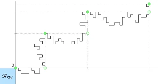
Proposition 3.1 implies that the prudent walker behaves qualitatively, asymptotically, in the same way as a simplified model in which the evolution is along the corner of the infinite rectangle
RSW :={(x,y)∈Z2:x≤0,y≤0}. Namely, redefine a direction~e∈ {±~e1,±~e2}to be allowed if
and only if{γt+k~e,k>0} ∩(γ[0,t]∪ RSW) =∅. The paths of the corner processγb·are obtained by choosing at each step a nearest neighbour, uniformly in the allowed directions. A trajectory of the corner model is depicted on Figure 4. As before,bγ·can be decomposed into a concatenation of excursions along the vertical and horizontal sides ofRSW, denoted respectivelyEbv
k,Eb
h
0
RSW
Figure 4: A trajectory of the corner processbγ·.
We relate the true excursions of the prudent walk to those of the corner model, by means of the following coupling. As before, we assume that the first step is horizontal: bγ1= (1, 0). Consider a given realisation of(Ebv
k,Eb
h
k)k≥1, from which we construct(Ekv,E
h
k)k≥1, with the same distribution
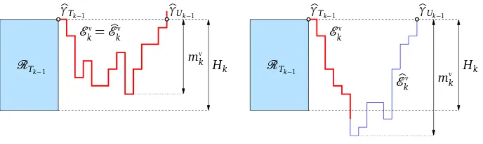
as the excursions of the prudent walk. Let (see Fig. 5)
mv restriction ofEbv
k up to timetℓ. Similarly, one defines the corresponding objects in the horizontal case. LetH0:=0 and set
LetX0be the horizontal displacement associated toEv
1as in Figure 3, and setW0=X0. We then
j)j=1,...,k have already been defined. To each vertical excursionEjv, we associate a horizontal displacementXjas in Figure 3. Similarly, to each horizontal excursionEjh, we associate a vertical displacementYj.
SetHk:=Y0+· · ·+Yk−1, and
Hk
Figure 5: The construction of the vertical excursionEv
kofγ·from the vertical excursionEbkv ofγb·.
WhenEbv
kis compatible withRTk−1, it is kept (left); when it is not compatible, it is truncated (right).
(Ev
k,E
h
k)k≥1is distributed exactly as the excursions of the true prudent walk up to the appropriate
reflection. By Proposition 3.1, almost surely,Eh
k=Eb According to Proposition 3.1, the prudent walkerγ·eventually fixates in one of the four quadrants and couples with the trajectory of the corner model γˆ·. Obvious lattice symmetries present in the model imply that the quadrant is chosen with uniform probability 1/4. In order to lighten notations, we shall assume that the chosen quadrant is the first one.
Theorem 3.1. Let us denote byQ1 the event thatγ· eventually settles in the first quadrant; notice that P(Q1) =1/4. We then have, for anyε >0,
Proof. By Proposition 3.1,γ·andbγ·couple almost surely in finite time. Since, onQ1, the distance between the two processes (at the same time) remains constant after coupling, it follows that, almost surely, supt≥0kbγt−γtk1<∞.
4
The scaling limit: Proof of Theorem 1.1
Theorem 1.1 is a consequence of Theorem 3.1 and the following result.
Theorem 4.1. On a suitably enlarged probability space, one can construct simultaneously a realiza-tion ofbγ·and of a Brownian motion W·such that, for anyε >0,
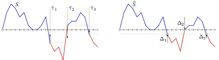
The rest of this section is devoted to the proof of Theorem 4.1. We start by establishing a suitable coupling between the corner process and the effective random walk S· introduced in Subsec-tion 2.1. To this end, we construct a process Sˆ· associated to the effective random walkS·. This construction is illustrated on Figure 6.
τ2
τ1 τ3
∆1 ∆2
∆3
S· bS·
Figure 6: The construction of the processSˆ·.
Observe thatτk+1−τkhas the same distribution asη∞. Define the overshoots as∆0:=0, and for
allk∈Z≥0,
∆2k+1:=−1−(Sτ2k+1−Sτ2k),
∆2k+2:= +1−(Sτ2k+2−Sτ2k+1).
Thanks to the memoryless property of the geometric distribution, we have that, for allk,(−1)k+1∆
k is a non-negative random variable, with geometric distribution of parameter 1/2. We now define
b
Sn:=Sn+
X
j≥0
∆j1{τj≤n}. (9)
The trajectory of the corner model can be constructed from the processbS·, by decomposing the trajectory of the latter into two types of “excursions”: those starting at 0 and ending at−1, and those starting at−1 and ending at 0. Applying the inverse of the procedure described in Fig. 3 to an excursion of the first type, we construct a vertical excursion ofbγ·; similarly, applying the same procedure to an excursion of the second type, we construct a horizontal excursion ofγb·. The fact that these have the proper distribution follows from Lemma 2.1.
The next result shows that the sup-norm between the two processesS·andSb·up to any fixed time never gets too large.
Lemma 4.1. For anyδ >0,
lim
n→∞P 0max≤k≤n|Sk−bSk| ≥n
1/4+δ=0.
Proof. By (9), we haveSk−Sbk=S˜No(k)−∆k+1/2, where ˜SN:=
PN
j=0∆˜i, ˜∆i:= (∆i+ ∆i+1)/2 and No(k):=max
¦
j≥0 :τj≤k©. Observe that the random variables ˜∆iare i.i.d. and symmetric; in particular, ˜SN is a martingale. IfL:=n1/4+δ,
lim
n→∞P 0max≤k≤n|Sk−Sbk| ≥n
1/4+δ
≤ lim
n→∞P maxk≤n| ˜
SNo(k)| ≥L/2
≤ lim
n→∞P j≤maxNo(n)
|S˜j| ≥L/2
≤ lim
n→∞P maxj≤L2|
˜
Sj| ≥L/2+ lim
n→∞P(No(n)≥L 2).
Lemma 4.2. Fix1/8> δ >0. For allε >0, we have
The next ingredient is the existence of a strong coupling between the effective random walk S·
and the Brownian motionB·[7]: on a suitably enlarged probability space, we can construct both processes in such a way that, fornlarge enough,
Let us now introduce Using these notations, we can deduce from Lemmas 4.2 and 4.3 that
lim
Snis mapped on the pointbγt(n)by the transformation described before Lemma 4.1.
Lemma 4.4. For anyε >0,
we deduce that
To sum up, we have established that, for allε >0,
lim
In the present work, we have focused on some of the most striking features of the scaling limit of the (kinetic) prudent walk. There remain however a number of open problems. We list a few of them here.
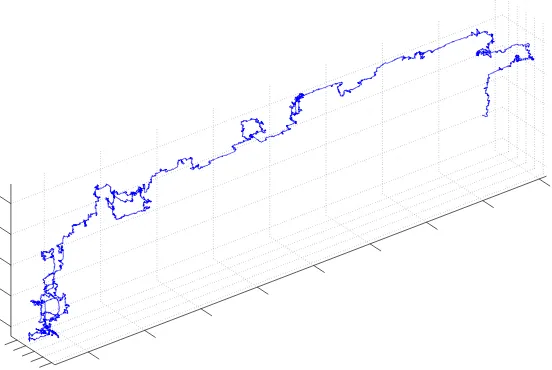
• It would be interesting to determine the scaling limit of the prudent walk on other lattices, e.g., triangular. Observe that the scaling limit we obtain reflects strongly the symmetries of the Z2 lattice, and is thus very likely to be different for other lattices. Nevertheless, numerical simulations indicate that similar scaling limits hold.
Figure 7: A trajectory of a 3-dimensional generalization of the prudent walk (first variant) with 6 million steps.
The second variant is easier, and it is likely to be in the scope of a suitable extension of our techniques. The first variant, however, is much more subtle (and interesting). Numerical simulations suggest the existence of an anomalous scaling exponent: Ifγt is the location of the walk aftertsteps, its norm appears to be of ordertαwithα≃.75 (but we see no reason to expectαto be equal to 3/4).
• Derive the scaling limit of the uniform prudent walk. In particular, it was observed numeri-cally[3]that the number of prudent walks has the same growth rate as that of the (explicitly computed) number of so-called 2-sided prudent walks (which are somewhat analogous to our corner model). This should not come as a surprise, since one expects the uniform pru-dent walk to visit all corners but one only finitely many times. It would be interesting to see whether it is possible to make sense of the fact that the uniform prudent walk is more strongly concentrated along (one of) the diagonal. This would permit to derive a proof of the previous result from the one of the kinetic model.
References
[1] O. Angel, I. Benjamini, and B. Virág. Random walks that avoid their past convex hull.
Electron. Comm. Probab., 8:6–16 (electronic), 2003. MR1961285
[2] M. Bousquet-Mélou. Families of prudent self-avoiding walks. Preprint arXiv: 0804.4843.
[4] J. C. Dethridge and A. J. Guttmann. Prudent self-avoiding walks. Entropy, 10:309–318, 2008. MR2465840
[5] E. Duchi. On some classes of prudent walks. FPSAC ’05, Taormina, Italy, 2005.
[6] A. J. Guttmann. Some solvable, and as yet unsolvable, polygon and walk models. Inter-national Workshop on Statistical Mechanics and Combinatorics: Counting Complexity, 42:98– 110, 2006.
[7] J. Komlós, P. Major, and G. Tusnády. An approximation of partial sums of independent RV’s, and the sample DF. II. Z. Wahrscheinlichkeitstheorie und Verw. Gebiete, 34(1):33–58, 1976. MR0402883
[8] G. F. Lawler and V. Limic. Random Walk: a Modern Introduction. Preliminary draft (version: February 2010).
[9] S. B. Santra, W. A. Seitz, and D. J. Klein. Directed self-avoiding walks in random media.
Phys. Rev. E, 63(6):067101, Part 2 JUN 2001.
[10] U. Schwerdtfeger. Exact solution of two classes of prudent polygons. Preprint arXiv: 0809.5232.
[11] L. Turban and J.-M. Debierre. Self-directed walk: a Monte Carlo study in three dimensions.
J. Phys. A, 20:3415–3418, 1987. MR0914064
[12] L. Turban and J.-M. Debierre. Self-directed walk: a Monte Carlo study in two dimensions.J. Phys. A, 20:679–686, 1987. MR0914064