El e c t ro n ic
Jo ur
n a l o
f P
r o
b a b il i t y
Vol. 16 (2011), Paper no. 2, pages 45–75. Journal URL
http://www.math.washington.edu/~ejpecp/
Can the adaptive Metropolis algorithm collapse without
the covariance lower bound?
∗
Matti Vihola
Department of Mathematics and Statistics University of Jyväskylä
P.O.Box 35
FI-40014 University of Jyväskyla Finland
http://iki.fi/mvihola/
Abstract
The Adaptive Metropolis (AM) algorithm is based on the symmetric random-walk Metropolis algorithm. The proposal distribution has the following time-dependent covariance matrix at step n+1
Sn=Cov(X1, . . . ,Xn) +εI,
that is, the sample covariance matrix of the history of the chain plus a (small) constantε >0 multiple of the identity matrixI. The lower bound on the eigenvalues ofSninduced by the factor
εI is theoretically convenient, but practically cumbersome, as a good value for the parameter
εmay not always be easy to choose. This article considers variants of the AM algorithm that do not explicitly bound the eigenvalues ofSn away from zero. The behaviour ofSn is studied
in detail, indicating that the eigenvalues ofSn do not tend to collapse to zero in general. In
dimension one, it is shown thatSnis bounded away from zero if the logarithmic target density
is uniformly continuous. For a modification of the AM algorithm including an additional fixed ∗The author was supported by the Academy of Finland, projects no. 110599 and 201392, by the Finnish Academy
component in the proposal distribution, the eigenvalues ofSnare shown to stay away from zero with a practically non-restrictive condition. This result implies a strong law of large numbers for super-exponentially decaying target distributions with regular contours.
Key words: Adaptive Markov chain Monte Carlo, Metropolis algorithm, stability, stochastic ap-proximation.
AMS 2000 Subject Classification:Primary 65C40.
1
Introduction
Adaptive Markov chain Monte Carlo (MCMC) methods have attracted increasing interest in the last few years, after the original work of Haario, Saksman, and Tamminen Haario et al. (2001) and the subsequent advances in the field Andrieu and Moulines (2006); Andrieu and Robert (2001); Atchadé and Rosenthal (2005); Roberts and Rosenthal (2007); see also the recent review Andrieu and Thoms (2008). Several adaptive MCMC algorithms have been proposed up to date, but the seminal Adaptive Metropolis (AM) algorithm Haario et al. (2001) is still one of the most applied methods, perhaps due to its simplicity and generality.
The AM algorithm is a symmetric random-walk Metropolis algorithm, with an adaptive proposal distribution. The algorithm starts1 at some point X1 ≡ x1 ∈ Rd with an initial positive definite covariance matrixS1≡s1∈Rd×d and follows the recursion
(S1) LetYn+1=Xn+θS1/2n Wn+1, whereWn+1 is an independent standard Gaussian random vector
andθ >0 is a constant.
(S2) Accept Yn+1 with probability min
1,π(Yn+1)
π(Xn) and let Xn+1 =Yn+1; otherwise rejectYn+1 and
letXn+1=Xn.
(S3) SetSn+1= Γ(X1, . . . ,Xn+1).
In the original work Haario et al. (2001) the covariance parameter is computed by
Γ(X1, . . . ,Xn+1) =
1 n
n+1
X
k=1
(Xk−Xn+1)(Xk−Xn+1)T +εI, (1)
where Xn := n−1
Pn
k=1Xk stands for the mean. That is, Sn+1 is a covariance estimate of the
history of the ‘Metropolis chain’ X1, . . . ,Xn+1 plus a small ε > 0 multiple of the identity matrix
I ∈ Rd×d. The authors prove a strong law of large numbers (SLLN) for the algorithm, that is, n−1Pnk=1f(Xk)→R
Rdf(x)π(x)dx almost surely asn→ ∞for any bounded functional f when the
target distributionπis bounded and compactly supported. Recently, SLLN was shown to hold also forπwith unbounded support, having super-exponentially decaying tails with regular contours and
f growing at most exponentially in the tails Saksman and Vihola (2010).
This article considers the original AM algorithm (S1)–(S3), without the lower bound induced by the factorεI. The proposal covariance function Γ, defined precisely in Section 2, is a consistent covariance estimator first proposed in Andrieu and Robert (2001). A special case of this estimator behaves asymptotically like the sample covariance in (1). Previous results indicate that if this algo-rithm is modified by truncating the eigenvalues ofSn within explicit lower and upper bounds, the algorithm can be verified in a fairly general setting Atchadé and Fort (2010); Roberts and Rosenthal (2007). It is also possible to determine an increasing sequence of truncation sets forSn, and mod-ify the algorithm to include a re-projection scheme in order to vermod-ify the validity of the algorithm Andrieu and Moulines (2006).
While technically convenient, such pre-defined bounds on the adapted covariance matrixSn can be inconvenient in practice. Ill-defined values can affect the efficiency of the adaptive scheme dramat-ically, rendering the algorithm useless in the worst case. In particular, if the factorε >0 in the AM
algorithm is selected too large, the smallest eigenvalue of the true covariance matrix ofπ may be well smaller than ε > 0, and the chain Xn is likely to mix poorly. Even though the re-projection
scheme of Andrieu and Moulines (2006) avoids such behaviour by increasing truncation sets, which eventually contain the desirable values of the adaptation parameter, the practical efficiency of the algorithm is still strongly affected by the choice of these sets Andrieu and Thoms (2008).
Without a lower bound on the eigenvalues ofSn (or a re-projection scheme), there is a potential
danger of the covariance parameter Sn collapsing to singularity. In such a case, the increments Xn−Xn−1would be smaller and smaller, and theXnchain could eventually get ‘stuck’. The empirical evidence suggests that this does not tend to happen in practice. The present results validate the empirical findings by excluding such a behaviour in different settings.
After defining precisely the algorithms in Section 2, the above mentioned unconstrained AM algo-rithm is analysed in Section 3. First, the AM algoalgo-rithm run on an improper uniform targetπ≡c>0 is studied. In such a case, the asymptotic expected growth rate ofSnis characterised quite precisely, beinge2θpnfor the original AM algorithm Haario et al. (2001). The behaviour of the AM algorithm in the uniform target setting is believed to be similar as in a situation whereSn is small and the target πis smooth whence locally constant. The results support the strategy of choosing a ‘small’ initial covariances1 in practice, and letting the adaptation take care of expanding it to the proper
size.
In Section 3, it is also shown that in a one-dimensional setting and with a uniformly continuous logπ, the variance parameterSn is bounded away from zero. This fact is shown to imply, with the results in Saksman and Vihola (2010), a SLLN in the particular case of a Laplace target distribution. While this result has little practical value in its own right, it is the first case where the unconstrained AM algorithm is shown to preserve the correct ergodic properties. It shows that the algorithm possesses self-stabilising properties and further strengthens the belief that the algorithm would be stable and ergodic under a more general setting.
Section 4 considers a slightly different variant of the AM algorithm, due to Roberts and Rosenthal Roberts and Rosenthal (2009), replacing (S1) with
(S1’) With probabilityβ, letYn+1 =Xn+Vn+1 where Vn+1 is an independent sample ofqfix;
other-wise, letYn+1=Xn+θSn1/2Wn+1 as in (S1).
While omitting the parameterε >0, the proposal strategy (S1’) includes two additional parameters: the mixing probability β ∈ (0, 1) and the fixed symmetric proposal distribution qfix. It has the
2
The general algorithm
Let us define a Markov chain(Xn,Mn,Sn)n≥1 evolving in spaceRd×Rd× Cd with the state space
Rd andCd⊂Rd×dstanding for the positive definite matrices. The chain starts at an initial position X1 ≡ x1∈Rd, with an initial mean2 M1 ≡m1∈Rd and an initial covariance matrixS1≡s1∈ Cd.
Forn≥1, the chain is defined through the recursion
Xn+1 ∼ PqSn(Xn,·) (2)
Mn+1 := (1−ηn+1)Mn+ηn+1Xn+1 (3)
Sn+1 := (1−ηn+1)Sn+ηn+1(Xn+1−Mn)(Xn+1−Mn)T. (4)
Denoting the natural filtration of the chain asFn :=σ(Xk,Mk,Sk : 1≤k≤n), the notation in (2) reads that PXn+1∈A
Fn
= PqSn(Xn,A)for any measurableA⊂Rd. The Metropolis transition
kernelPqis defined for any symmetric probability densityq(x,y) =q(x−y)through
Pq(x,A):=1A(x)
1−
Z
min
1,π(y) π(x)
q(y−x)dy
+
Z
A
min
1,π(y) π(x)
q(y−x)dy
where 1A stands for the characteristic function of the set A. The proposal densities {qs}s
∈Cd are
defined as a mixture
qs(z):= (1−β)q˜s(z) +βqfix(z) (5)
where the mixing constant β ∈ [0, 1) determines the portion how often a fixed proposal density qfix is used instead of the adaptive proposal ˜qs(z) := det(θs)−1/2˜q(θ−1/2s−1/2z) with ˜q being a ‘template’ probability density. Finally, the adaptation weights(ηn)n≥2⊂(0, 1)appearing in (3) and
(4) is assumed to decay to zero.
One can verify that forβ=0 this setting corresponds to the algorithm (S1)–(S3) of Section 1 with Wn+1 having distribution ˜q, and forβ ∈(0, 1), (S1’) applies instead of (S1). Notice also that the
original AM algorithm essentially fits this setting, withηn:=n−1,β:=0 and if ˜qsis defined slightly
differently, being a Gaussian density with mean zero and covariances+εI. Moreover, if one sets β =1, the above setting reduces to a non-adaptive symmetric random walk Metropolis algorithm with the increment proposal distributionqfix.
3
The unconstrained AM algorithm
3.1
Overview of the results
This section deals with the unconstrained AM algorithm, that is, the algorithm described in Section 2 with the mixing constantβ=0 in (5). Sections 3.2 and 3.3 consider the case of an improper uniform target distributionπ≡cfor some constantc>0. This implies that (almost) every proposed sample is accepted and the recursion (2) reduces to
Xn+1=Xn+θSn1/2Wn+1 (6)
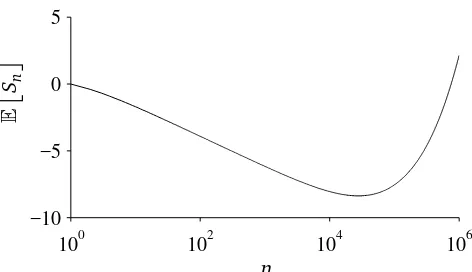
100 102 104 106 −10
−5 0 5
E
Sn
n
Figure 1: An example of the exact development ofE
Sn
, whens1=1 andθ=0.01. The sequence
(E
Sn
)n≥1decreases untilnis over 27, 000 and exceeds the initial value only withnover 750, 000.
where(Wn)n≥2are independent realisations of the distribution ˜q.
Throughout this subsection, let us assume that the template proposal distribution ˜q is spherically symmetric and the weight sequence is defined as ηn := cn−γ for some constants c ∈ (0, 1] and
γ∈(1/2, 1]. The first result characterises the expected behaviour ofSn when(Xn)n≥2follows (6).
Theorem 1. Suppose(Xn)n≥2 follows the ‘adaptive random walk’ recursion (6), with EWnWnT = I .
Then, for allλ >1there is n0≥m such that for all n≥n0and k≥1, the following bounds hold
1 λ
θ
n+k
X
j=n+1
p
ηj
≤log
ESn+k
ESn
≤λ
θ
n+k
X
j=n+1
p
ηj
.
Proof. Theorem 1 is a special case of Theorem 12 in Section 3.2.
Remark2. Theorem 1 implies that with the choice ηn:=cn−γ for somec∈(0, 1)andγ∈(1/2, 1],
the expectation grows with the speed
ESn
≃exp θ
p
c
1−γ2n
1−γ2
!
.
Remark 3. In the original setting (Haario et al. 2001) the weights are defined as ηn := n−1 and
Theorem 1 implies that the asymptotic growth rate of E[Sn] is e2θpn when (Xn)n≥2 follows (6). Suppose the value ofSnis very small compared to the scale of a smooth target distributionπ. Then,
it is expected that most of the proposal are accepted,Xn behaves almost as (6), andSn is expected to grow approximately at the ratee2θpn until it reaches the correct magnitude. On the other hand, simple deterministic bound implies thatSn can decay slowly, only with the polynomial speed n−1.
Therefore, it may be safer to choose the initials1 small.
It may seem that Theorem 1 would automatically also ensure thatSn → ∞also path-wise. This is not, however, the case. For example, consider the probability space[0, 1]with the Borelσ-algebra and the Lebesgue measure. Then(Mn,Fn)n≥1 defined as Mn :=22n1[0,2−n) andFn :=σ(X
k : 1≤
k≤n)is, in fact, a submartingale. Moreover,EMn=2n→ ∞, but Mn→0 almost surely.
The AM process, however, does produce an unbounded sequenceSn.
Theorem 5. Assume that(Xn)n≥2follows the ‘adaptive random walk’ recursion(6). Then, for any unit
vector u∈Rd, the process uTSnu→ ∞almost surely.
Proof. Theorem 5 is a special case of Theorem 18 in Section 3.3.
In a one-dimensional setting, and when logπ is uniformly continuous, the AM process can be ap-proximated with the ‘adaptive random walk’ above, wheneverSn is small enough. This yields
Theorem 6. Assume d =1and logπ is uniformly continuous. Then, there is a constant b>0such
thatlim infn→∞Sn≥b.
Proof. Theorem 6 is a special case of Theorem 18 in Section 3.4.
Finally, having Theorem 6, it is possible to establish
Theorem 7. Assumeq is Gaussian, the one-dimensional target distribution is standard Laplace˜ π(x):=
1 2e−|
x| and the functional f : R → R satisfies sup
xe−γ|x||f(x)| < ∞ for some γ∈ (0, 1/2). Then,
n−1Pnk=1f(Xk)→R f(x)π(x)dx almost surely as n→ ∞.
Proof. Theorem 7 is a special case of Theorem 21 in Section 3.4.
Remark8. In the caseηn := n−1, Theorem 7 implies that the parameters Mn andSn of the
adap-tive chain converge to 0 and 2, that is, the true mean and variance of the target distribution π, respectively.
Remark 9. Theorem 6 (and Theorem 7) could probably be extended to cover also targets π with compact supports. Such an extension would, however, require specific handling of the boundary effects, which can lead to technicalities.
3.2
Uniform target: expected growth rate
Define the following matrix quantities
an := E
(Xn−Mn−1)(Xn−Mn−1)T
(7)
bn := E
Sn
(8)
forn≥1, with the convention thata1≡0∈Rd×d. One may write using (3) and (6) Xn+1−Mn=Xn−Mn+θS1/2n Wn+1= (1−ηn)(Xn−Mn−1) +θS1/2n Wn+1.
IfEWnWnT =I, one may easily compute
E
(Xn+1−Mn)(Xn+1−Mn)T
= 1−ηn
2
sinceWn+1 is independent ofFn and zero-mean due to the symmetry of ˜q. The values of (an)n≥2 and(bn)n≥2are therefore determined by the joint recursion
an+1 = (1−ηn)2an+θ2bn (9)
bn+1 = (1−ηn+1)bn+ηn+1an+1. (10)
Observe that for any constant unit vectoru∈Rd, the recursions (9) and (10) hold also for
a(nu+)1 := EuT(Xn+1−Mn)(Xn+1−Mn)Tu
b(nu+)1 := EuTSn+1u
.
The rest of this section therefore dedicates to the analysis if the one-dimensional recursions (9) and (10), that is,an,bn∈R+for alln≥1. The first result shows that the tail of(bn)n≥1 is increasing.
Lemma 10. Let n0≥1and suppose an0≥0, bn0>0and for n≥n0the sequences anand bnfollow the
recursions(9)and(10), respectively. Then, there is a m0≥n0such that(bn)n≥m
0is strictly increasing.
Proof. Ifθ ≥1, we may estimate an+1 ≥(1−ηn)2an+bn implying bn+1 ≥ bn+ηn+1(1−ηn)2an
for all n≥ n0. Since bn > 0 by construction, and therefore also an+1 ≥ θ2bn > 0, we have that
bn+1> bnfor alln≥n0+1.
Suppose thenθ <1. Solvingan+1 from (10) yields
an+1=η−n+11 bn+1−bn
+bn
Substituting this into (9), we obtain forn≥n0+1
η−n+11 bn+1−bn
+bn= (1−ηn)2
η−n1 bn−bn−1
+bn−1
+θ2bn
After some algebraic manipulation, this is equivalent to
bn+1−bn=
ηn+1
ηn
(1−ηn)3(bn−bn−1) +ηn+1
(1−ηn)2−1+θ2
bn. (11)
Now, sinceηn→0, we have that(1−ηn)2−1+θ2>0 whenevernis greater than somen1. So, if
we have for somen′>n1 that bn′−bn′−1≥0, the sequence(bn)n≥n′ is strictly increasing aftern′. Suppose conversely that bn+1−bn < 0 for all n≥ n1. From (10), bn+1− bn = ηn+1(an+1− bn)
and hence bn > an+1 forn≥n1. Consequently, from (9), an+1 > (1−ηn)2an+θ2an+1, which is
equivalent to
an+1> (1−ηn)
2
1−θ2 an.
Sinceηn→0, there is aµ >1 andn2such thatan+1≥µanfor alln≥n2. That is,(an)n≥n2 grows at least geometrically, implying that after some timean+1>bn, which is a contradiction. To conclude, there is anm0≥n0 such that(bn)n≥m0 is strictly increasing.
Lemma 10 shows that the expectationEuTSnuis ultimately bounded from below, assuming only thatηn →0. By additional assumptions on the sequenceηn, the growth rate can be characterised
Assumption 11. Suppose(ηn)n≥1⊂(0, 1)and there ism′≥2 such that
(i) (ηn)n≥m′ is decreasing withηn→0,
(ii) (η−n+1/21 −η−n1/2)n≥m′ is decreasing and
(iii) P∞n=2ηn=∞.
The canonical example of a sequence satisfying Assumption 11 is the one assumed in Section 3.1, ηn:=cn−γforc∈(0, 1)andγ∈(1/2, 1].
Theorem 12. Suppose am ≥0and bm> 0for some m≥1, and for n>m the an and bn are given
recursively by(9)and (10), respectively. Suppose also that the sequence(ηn)n≥2 satisfies Assumption
11 with some m′ ≥m. Then, for allλ >1there is m2≥ m′ such that for all n≥ m2 and k≥1, the
Proof. Let m0 be the index from Lemma 10 after which the sequence bn is increasing. Let m1 > max{m0,m′}and define the sequence(zn)n≥m1−1 by settingzm1−1 =bm1−1 andzm1 = bm1, and for
n≥m1through the recursion
Letλ′>1. Since gn(1)→θ˜(1) and gn(2)→θ˜(2) there is a m2 ≥ m1 such that the following bounds
Similarly, by the mean value theorem
log
sinceηnis decreasing. By letting the constantm1above be sufficiently large, the difference|θ˜(2)−θ|
can be made arbitrarily small, and by increasing m2, the constantλ′>1 can be chosen arbitrarily
close to one.
3.3
Uniform target: path-wise behaviour
Section 3.2 characterised the behaviour of the sequenceE
Sn
when the chain(Xn)n≥2 follows the
‘adaptive random walk’ recursion (6). In this section, we shall verify that almost every sample path (Sn)n≥1of the same process are increasing.
Let us start by expressing the processSnin terms of an auxiliary process(Zn)n≥1.
Lemma 13. Let u∈Rd be a unit vector and suppose the process(Xn,Mn,Sn)n≥1is defined through(3),
(4)and (6), where(Wn)n≥1 are i.i.d. following a spherically symmetric, non-degenerate distribution.
Define the scalar process(Zn)n≥2through
The proof of Lemma 13 is given in Appendix B.
It is immediate from (14) that only values|Zn|<1 can decreaseuTSnu. On the other hand, if both ηnandηnZn2 are small, then the variableUnis clearly close to unity. This suggests a nearly random
walk behaviour of Zn. Let us consider an auxiliary result quantifying the behaviour of this random
Lemma 14. Let n0 ≥ 2, suppose Z˜n
0−1 isFn0−1-measurable random variable and suppose(W˜n)n≥n0
are respectively (Fn)n≥n
0-measurable and non-degenerate i.i.d. random variables. Define for Z˜n for
n≥2through
Proof. From the Kolmogorov-Rogozin inequality, Theorem 36 in Appendix C,
P(Z˜n+j−Z˜n∈[x,x+2N]| Fn)≤c1j−1/2
The technical estimate in the next Lemma 16 makes use of the above mentioned random walk approximation and guarantees ultimately a positive ‘drift’ for the eigenvalues of Sn. The result requires that the adaptation sequence (ηn)n≥2 is ‘smooth’ in the sense that the quotients converge
Proof. Fix aγ∈(0, 2/3). Define the setsAn:j:=∩ij=n+1{Zi2≤η−i γ}andA′i:={Zi2> η−i γ}. Write the conditional expectation in parts as follows,
PLn,k
whenevern≥n0is sufficiently large, sinceηn→0, and by Assumption 15. That is, ifnis sufficiently
large, all but the first term in the right hand side of (16) are a.s. zero. It remains to show the inequality for the first.
by the mean value theorem, where the constantβj =βj(C,ηj)∈(0, 1) can be selected arbitrarily
small whenever jis sufficiently large. Using this estimate, one can write forω∈An:n+k
k
for sufficiently largen≥1, as then the constantβn can be chosen small enough, and by Assumption
15. In other words, ifn≥1 is sufficiently large, thenBn,k∩An:n+k∩Ln,k=;. Now, Lemma 14 yields
Using the estimate of Lemma 16, it is relatively easy to show that uTSnutends to infinity, if the adaptation weights satisfy an additional assumption.
Assumption 17. The adaptation weight sequence(ηn)n≥2⊂(0, 1)is inℓ2 but not inℓ1, that is,
Theorem 18. Assume that (Xn)n≥2 follows the ‘adaptive random walk’ recursion (6)and the
adap-tation weights(ηn)n≥2 satisfy Assumptions 15 and 17. Then, for any unit vector u∈Rd, the process
uTSnu→ ∞almost surely.
Proof. The proof is based on the estimate of Lemma 16 applied with a similar martingale argument as in Vihola (2009).
with the convention thatη0 =1. Form a martingale(Yi,Gi)i≥1 withY1 ≡0 and having differences
dYi :=Ti−E
Ti
Gi−1
and whereG1≡ {;,Ω}andGi:=Fℓ
i fori≥1. By Assumption 17,
∞
X
i=2
EdYi2≤c
∞
X
i=1
η2ℓ
i <∞
with a constantc=c(k,C)>0, soYi is aL2-martingale and converges a.s. to a finite limitM∞(e.g. Hall and Heyde 1980, Theorem 2.15).
By Lemma 16, the conditional expectation satisfies
ETi+1
Gi
≥kCηℓi(1−ε) + ℓi+1
X
j=ℓi+1
log(1−ηj)ε≥kηℓi
when i is large enough, and where the second inequality is due to Assumption 15. This implies, with Assumption 17, thatPiETi Gi−1
=∞a.s., and sinceYi converges a.s. to a finite limit, it holds thatPiTi =∞a.s.
By (14), one may estimate for anyn=ℓm withm≥1 that
log(uTSnu)≥log(uTS1u) + m
X
i=1
Ti→ ∞
asm→ ∞. Simple deterministic estimates conclude the proof for the intermediate values ofn.
3.4
Stability with one-dimensional uniformly continuous log-density
In this section, the above analysis of the ‘adaptive random walk’ is extended to imply that lim infn→∞Sn > 0 for the one-dimensional AM algorithm, assuming logπ uniformly continuous. The result follows similarly as in Theorem 18, by coupling the AM process with the ‘adaptive ran-dom walk’ wheneverSnis small enough to ensure that the acceptance probability is sufficiently close to one.
Theorem 19. Assume d = 1 and logπ is uniformly continuous, and that the adaptation weights
(ηn)n≥2satisfy Assumptions 15 and 17. Then, there is a constant b>0such thatlim infn→∞Sn≥ b.
Proof. Fix aδ∈(0, 1). Due to the uniform continuity of logπ, there is a ˜δ >0 such that
logπ(y)−logπ(x)≥ 1 2log
1−δ 2
for all|x− y| ≤δ˜1. Choose ˜M >0 sufficiently large so that
R
{|z|≤M˜}q˜(z)dz≥
p
1−δ/2. Denote by
Qq(x,A):=
Z
A
the random walk transition kernel with increment distribution q, and observe that the ‘adaptive
Define also ˜Ti similarly as Ti, but having ˜Z
Consequently, denotingGi:=Fℓi, Lemma 16 guarantees that
P
Let us show next that wheneverSℓi−1 is small, the variable Ti is expected to have a positive value proportional to the adaptation weight,
ETi
almost surely for any sufficiently largei≥1. Write first
ETi Gi−1
for any sufficiently largei. On the other hand, ifP
This establishes (20).
Define the stopping timesτ1≡1 and forn≥2 throughτn:=inf{i> τn−1:Sℓi−1≥µ/2,Sℓi < µ/2}
with the convention that inf;= ∞. That is,τi record the times when Sℓi enters (0,µ/2]. Using
τi, define the latest such time up to n by σn := sup{τi : i ≥ 1,τi ≤ n}. As in Theorem 18, define the almost surely converging martingale(Yi,Gi)i≥1 with Y1 ≡0 and having the differences dYi := (Ti−E
Ti
Gi−1
)fori≥2.
It is sufficient to show that lim infi→∞Sℓ
i ≥ b:= µ/4>0 almost surely. If there is a finite i0 ≥1
such thatSℓi ≥µ/2 for alli≥i0, the claim is trivial. Let us consider for the rest of the proof the case
that{Sℓi < µ/2}happens for infinitely many indicesi≥1.
For anym≥2 such thatSℓm< µ/2, one can write
logSℓm≥logSℓσm+ m
X
i=σm+1
Ti
≥logSℓσm+ (Ym−Yσm) + m
X
i=σm+1
kηℓi−1
(21)
since thenSℓ
i < µ/2 for alli∈[σm,m−1]and hence alsoE
Ti Gi−1
≥kηℓi−1.
Suppose for a moment that there is a positive probability thatSℓm stays within(0,µ/2)indefinitely,
starting from some indexm1≥1. Then, there is an infiniteτi and consequentlyσm≤σ <∞for
allm≥1. But asYmconverges, |Ym−Yσm|is a.s. finite, and since
P
mηℓm=∞by Assumptions 15
and 17, the inequality (21) implies thatSℓm≥µ/2 for sufficiently largem, which is a contradiction.
That is, the stopping timesτi for all i≥ 1 must be a.s. finite, wheneverSℓm < µ/2 for infinitely
many indicesm≥1.
For the rest of the proof, supposeSℓm < µ/2 for infinitely many indicesm≥1. Observe that since
Ym → Y∞, there exists an a.s. finite index m2 so that Ym−Y∞ ≥ −1/2 log 2 for all m ≥ m2. As ηn→0 andσm→ ∞, there is an a.s. finitem3 such thatξσm−1 ≥ −1/2 log 2 for allm≥m3. For all
m≥max{m2,m3}and wheneverSℓm< µ/2, it thereby holds that
logSℓm≥logSℓσm −(Ym−Yσm)≥logSℓσm−1+ξσm− 1 2log 2
≥logµ
2−log 2=logb.
The caseSℓ
m≥µ/2 trivially satisfies the above estimate, concluding the proof.
As a consequence of Theorem 19, one can establish a strong law of large numbers for the uncon-strained AM algorithm running with a Laplace target distribution. Essentially, the only ingredient that needs to be checked is that the simultaneous geometric ergodicity condition holds. This is verified in the next lemma, whose proof is given in Appendix E.
Lemma 20. Suppose that the template proposal distribution ˜q is everywhere positive and
non-increasing away from the origin: ˜q(z) ≥ q˜(w) for all |z| ≤ |w|. Suppose also that π(x) :=
1
2bexp
constants M,b such that the following drift and minorisation condition are satisfied for all s≥ L and measurable A⊂R
PsV(x)≤λsV(x) +b1C(x), ∀x∈R (22)
Ps(x,A)≥δsν(A), ∀x ∈C (23)
where V :R→[1,∞)is defined as V(x):= (supzπ(z))1/2π−1/2(x), the set C := [m−M,m+M], the probability measureµis concentrated on C and PsV(x):=
R
V(y)Ps(x, dy). Moreover,λs,δs∈(0, 1)
satisfy for all s≥L
max{(1−λs)−1,δ−s1} ≤cs
γ (24)
for some constants c,γ >0that may depend on L.
Theorem 21. Assume the adaptation weights(ηn)n≥2satisfy Assumptions 15 and 17, and the template
proposal density˜q and the target distributionπsatisfy the assumptions in Lemma 20. If the functional f satisfiessupx∈Rπ−γ(x)|f(x)|<∞for someγ∈(0, 1/2). Then, n−1Pnk=1f(Xk)→
R
f(x)π(x)dx almost surely as n→ ∞.
Proof. The conditions of 19 are clearly satisfied implying that for anyε >0 there is aκ=κ(ε)>0 such that the event
Bκ:=
§
inf
n Sn≥κ
ª
has a probabilityP(Bκ)≥1−ε.
The inequalities (22) and (23) of Lemma 20 with the bound (24) imply, using (Saksman and Vihola 2010, Proposition 7 and Lemma 12), that for anyβ >0 there is a constantA=A(κ,ε,β)<∞such thatP(Bκ∩ {max{|Sn|,|Mn|}>Anβ})≤ε. Let us define the sequence of truncation sets
Kn:={(m,s)∈R×R+:λmin(s)≥κ, max{|s|,|m|} ≤Anβ}
for n≥ 1. Construct an auxiliary truncated process (X˜n, ˜Mn, ˜Sn)n≥1, starting from (X˜1, ˜M1, ˜S1) ≡ (X1,M1,S1)and forn≥2 through
˜
Xn+1 ∼ Pq˜Sn˜ (X˜n,·)
(M˜n+1, ˜Sn+1) = σn+1
h
(M˜n, ˜Sn),ηn+1 X˜n+1−M˜n,(X˜n+1−M˜n)2−S˜n
i
where the truncation functionσn+1:(Kn)×(R×R)→Knis defined as
σn+1(z,z′) =
(
z+z′, ifz+z′∈Kn z, otherwise.
Observe that this constrained process coincides with the AM process with probability P ∀n ≥ 1 : (X˜n, ˜Mn, ˜Sn) = (Xn,Mn,Sn)
4
AM with a fixed proposal component
This section deals with the modification due to Roberts and Rosenthal Roberts and Rosenthal (2009), including a fixed component in the proposal distribution. In terms of Section 2, the mixing parameter in (5) satisfies 0< β <1. Theorem 24 shows that the fixed proposal component guaran-tees, with a verifiable non-restrictive Assumption 22, that the eigenvalues of the adapted covariance parameterSnare bounded away from zero. As in Section 3.4, this result implies an ergodicity result, Theorem 29.
Let us start by formulating the key assumption that, intuitively speaking, assures that the adaptive chain(Xn)n≥1will have ‘uniform mobility’ regardless of the adaptation parameters∈ Cd.
Assumption 22. There exist a compactly supported probability measureν that is absolutely
contin-uous with respect to the Lebesgue measure, constantsδ >0 andc<∞and a measurable mapping ξ:Rd× Cd→Rd such that for allx ∈Rd ands∈ Cd,
kξ(x,s)−xk ≤c and Pqs(x,A)≥δν A−ξ(x,s)
for all measurable sets A⊂Rd, whereA− y :={x− y : x ∈A}is the translation of the set Aby y∈Rd.
Remark 23. In the case of the AM algorithm with a fixed proposal component, one is primarily interested in the case whereξ(x,s) =ξ(x)and for allx ∈Rd
βqfix(x−y)min
1,π(y) π(x)
≥δν y−ξ(x)
for all y∈Rd, whereν is a uniform density on some ball. Then, since Pqs = (1−β)P˜qs+βPqfix,
Pqs(x,A)≥βPqfix(x,A)≥δ
Z
A
ν(y−ξ)dy
and Assumption 22 is fulfilled by the measureν(A):=R
Aν(y)dy.
Having Assumption 22, the lower bound on the eigenvalues ofSn can be obtained relatively easily, by a martingale argument similar to the one used in Section 3 and in Vihola (2009).
Theorem 24. Let(Xn,Mn,Sn)n≥1 be an AM process as defined in Section 2 satisfying Assumption 22.
Moreover, suppose that the adaptation weights(ηn)n≥2satisfy Assumptions 15 and 17. Then,
lim inf
n→∞ winf∈Sdw TS
nw>0
whereSd stands for the unit sphere.
Proof. Let us first introduce independent binary auxiliary variables(Zn)n≥2withZ1≡0, and through
PZn+1=1 Xn,Mn,Sn,Zn
= δ
PZn+1=0
Xn,Mn,Sn,Zn
Using this auxiliary variable, we can assumeXnto follow3
Xn+1=Zn+1(Un+1+ Ξn) + (1−Zn+1)Rn+1
where Un+1 ∼ ν(·) is independent of Fn and Zn+1, the random variable Ξn := ξ(Xn,Sn) is Fn
-measurable, andRn+1 is distributed according to the ‘residual’ transition kernel ˇPS
n(Xn,A):= (1−
δ)−1[Pq
Sn(Xn,A)−δν(A−Ξn)], valid by Assumption 22.
DefineS(w,γ):={v∈ S d:kw−vk ≤γ}, the segment of the unit sphere centred atw∈ Sd and having the radiusγ >0. Fix a unit vectorw∈ Sd and define the following random variables
Γ(nγ+)2:= inf
v∈S(w,γ)
|vT(Xn+1−Mn)|2+|vT(Xn+2−Mn+1)|2
for all n ≥ 1. Denote Gn+1 := Xn+1−Mn and En+1 := Ξn+1−Xn+1, and observe that whenever
Zn+2=1, it holds that
Xn+2−Mn+1=Un+2+Xn+1−Mn+1+En+1
=Un+2+ (1−ηn+1)Gn+1+En+1
and we may write
Zn+2Γn(γ+)2=Zn+2 inf
v∈S(w,γ)
|vTGn+1|2+|vT(Un+2+λn+1Gn+1+En+1)|2
where λn :=1−ηn ∈(0, 1) for all n≥2. Consequently, we may apply Lemma 25 below to find
constantsγ,µ >0 such that
P
Zn+2Γ
(γ)
n+2≥µ
Fn
≥δ
2. (25)
Hereafter, assume γ > 0 is fixed such that (25) holds, and denote Γn+2 := Γ
(γ)
n+2 and S(w) := S(w,γ).
Consider the random variables
Dn+2:= inf
v∈S(w) ηn+1|v
T(X
n+1−Mn)|2+ηn+2|vT(Xn+2−Mn+1)|2
≥min{ηn+1,ηn+2}Γn+2≥η∗ηn+1Γn+2 (26)
whereη∗:=infk≥2ηk+1/ηk>0 by Assumption 15. Define the indicesℓn:=2n−1 forn≥1 and let
Tn:=η∗min{µ,ZℓnΓℓn}
for all n ≥ 2. Define the σ-algebras Gn := Fℓ
n for n ≥ 1 and observe that E
Tn+1 Gn
≥
η∗µδ/2 by (25). Construct a martingale starting fromY1 ≡0 and having the differences dYn+1 := ηℓn+1(Tn+1−E
Tn+1
Gn
). The martingaleYnconverges to an a.s. finite limitY∞as in Theorem
18.
Define alsoη∗:=supk≥2ηk+1/ηk<∞andκ:=infk≥21−ηk>0, and let
b:= κη∗µδ 8η∗ >0.
DenoteS(nw):=infv∈S(w)vTSnvand define the stopping timesτ1≡1 and fork≥2 through
As in the proof of Theorem 19, this is sufficient to find aǫ >0 such that
lim inf
n→∞ S
(w)
n ≥ǫ.
Finally, take a finite number of unit vectorsw1, . . . ,wN∈ Sd such that the corresponding segments
S(w1), . . . ,S(wN)coverSd. Then,
independent ofFn+1, having a distributionν fulfilling the conditions in Assumption 22.
LetSd:={u∈Rd:kuk=1}stand for the unit sphere and denote byS(w,γ):={v∈ Sd:kw−vk ≤ γ}the segment of the unit sphere centred at w∈ Sdand having the radiusγ >0. There exist constants
Proof. Sinceν is absolutely continuous with respect to the Lebesgue measure, one can show that
Corollary 26. Assume πis bounded, stays bounded away from zero on compact sets, is differentiable
on the tails, and has regular contours, that is,
lim inf weight satisfyingβ ∈(0, 1)and the density qfix is bounded away from zero in some neighbourhood of
the origin. Moreover, suppose that the adaptation weights (ηn)n≥2 satisfy Assumptions 15 and 17.
Then,
lim inf
n→∞ winf∈Sdw TS
nw>0.
Proof. In light of Theorem 24, it is sufficient to check Assumption 22, or in fact the conditions in Remark 23. Let L > 0 be sufficiently large so that infkxk≥L x
kxk · ∇π(x)
k∇π(x)k < 0. Jarner and Hansen
is contained in the setA(x):={y ∈Rd :π(y)≥π(x)}, for allkxk ≥L.
Let r′ >0 be sufficiently small to ensure that infkzk≤r′qfix(z)≥ δ′ > 0. There is a r = r(ε′,K) ∈ (0,r′/2) and measurable ξ: Rd →Rd such that kξ(x)−xk ≤ r′/2 and the ball B(x,r) := {y :
ky−ξ(x)k ≤r}is contained in the coneE(x). Define ν(x):=cr−11B(0,r)(x) where cr :=|B(0,r)|
is the Lebesgue measure ofB(0,r), and letξ(x):= x for the remainingkxk< L. Now, we have for
kxk ≥Lthat
βqfix(x− y)min
1,π(y) π(x)
≥βδ′crν(y−ξ).
Sinceπis bounded and bounded away from zero on compact sets, the ratioπ(y)/π(x)≥δ′′>0 for allx,y∈B(0,L+r′)withkx−yk ≤r′. Therefore, for allkxk<L, it holds that
βqfix(x−y)min
1,π(y) π(x)
≥βδ′δ′′crν(y−x).
Remark 27. The conditions of Corollary 26 are fulfilled by many practical densities π (see Jarner and Hansen (2000) for examples), and are fairly easy to verify in practice. Assumption 22 holds, however, more generally, excluding only densities with unbounded density or having irregular contours.
Remark28. It is not necessary for Theorem 24 and Corollary 26 to hold that the adaptive proposal densities {˜qs}s∈Cd have the specific form discussed in Section 2. The results require only that a
suitable fixed proposal component is used so that Assumption 22 holds. In Theorem 29 below, however, the structure of{q˜s}s∈Cd is required.
Let us record the following ergodicity result, which is a counterpart to (Saksman and Vihola 2010, Theorem 10) formulating a a strong law of large numbers for the original algorithm (S1)–(S3) with the covariance parameter (1).
Theorem 29. Suppose the target densityπis continuous and differentiable, stays bounded away from
zero on compact sets and has super-exponentially decaying tails with regular contours,
lim sup
kxk→∞
x
kxkρ· ∇logπ(x) =−∞ and lim sup
kxk→∞
x
kxk·
∇π(x)
k∇π(x)k <0,
respectively, for someρ >1.
Let(Xn,Mn,Sn)n≥1 be an AM process as defined in Section 2 using a mixture proposal qs(z) = (1−
β)q˜s(z) +βqfix(z) where q˜s stands for a zero-mean Gaussian density with covariance s, the mixing weight satisfiesβ∈(0, 1)and the density qfixis bounded away from zero in some neighbourhood of the origin. Moreover, suppose that the adaptation weights(ηn)n≥2satisfy Assumption 17.
Then, for any function f :Rd→Rwithsupx∈Rdπγ(x)|f(x)|<∞for someγ∈(0, 1/2),
1
n
n
X
k=1
f(Xk)−−−→n→∞
Z
Rd
f(x)π(x)dx
Proof. The conditions of Corollary 26 are satisfied, implying that for anyε >0 there is aκ=κ(ε)> 0 such thatP infnλmin(Sn) ≥κ
≥ 1−ε where λmin(s)denotes the smallest eigenvalue of s. By
(Saksman and Vihola 2010, Proposition 15), there is a compact setCκ⊂Rd, a probability measure
νκon Cκ, andbκ<∞such that for alls∈ Cd withλmin(s)≥κ, it holds that
P˜qsV(x)≤λsV(x) +b1C
κ(x), ∀x∈R
d (29)
P˜q
s(x,A)≥δsν(A) ∀x∈Cκ (30)
whereV(x):= (supxπ(x))1/2π−1/2(x)≥1 and the constantsλs,δs∈(0, 1)satisfy the bound
(1−λs)−1∨δs−1≤c1det(s)1/2 (31)
for some constant c1 ≥1. Likewise, there is a compactDf ⊂Rd, a probability measureµf on Df,
and constants bf <∞andλf,δf ∈(0, 1), so that (29) and (30) hold withPf (Jarner and Hansen
2000, Theorem 4.3). Put together, (29) and (30) hold for Pqs for all s ∈ C
d with λ
min(s) ≥ κ,
perhaps with different constants, but satisfying a bound (31), with anotherc2≥c1.
The rest of the proof follows as in Theorem 21 by construction of an auxiliary process(X˜n, ˜Mn, ˜Sn)n≥1 truncated so that for given ǫ > 0, κ ≤ λmin(S˜n) ≤ anǫ and |M˜n| ≤ anǫ and where the constant
a = a(ǫ,κ) is chosen so that the truncated process coincides with the original AM process with probability≥1−2ε. Theorem 2 of Saksman and Vihola (2010) ensures that the strong law of large numbers holds for the constrained process, and lettingε→0 implies the claim.
Remark 30. In the case ηn := n−1, Theorem 29 implies that with probability one, Mn → mπ :=
R
xπ(x)dx andSn→sπ:=R x xTπ(x)dx−mπmπT, the true mean and covariance ofπ, respectively.
Remark 31. Theorem 29 holds also when using multivariate Student distributions {˜qs}s∈Cd, as
(Vihola 2009, Proposition 26 and Lemma 28) extend the result in Saksman and Vihola (2010) to cover this case.
Acknowledgements
The author thanks Professor Eero Saksman for discussions and helpful comments on the manuscript.
References
C. Andrieu and É. Moulines. On the ergodicity properties of some adaptive MCMC algorithms. Ann. Appl. Probab., 16(3):1462–1505, 2006. MR2260070
C. Andrieu and C. P. Robert. Controlled MCMC for optimal sampling. Technical Report Ceremade 0125, Université Paris Dauphine, 2001.
C. Andrieu and J. Thoms. A tutorial on adaptive MCMC. Statist. Comput., 18(4):343–373, Dec. 2008. MR2461882
Y. F. Atchadé and J. S. Rosenthal. On adaptive Markov chain Monte Carlo algorithms. Bernoulli, 11 (5):815–828, 2005. MR2172842
K. B. Athreya and P. Ney. A new approach to the limit theory of recurrent Markov chains. Trans. Amer. Math. Soc., 245:493–501, 1978. MR0511425
Y. Bai, G. O. Roberts, and J. S. Rosenthal. On the containment condition for adaptive Markov chain Monte Carlo algorithms. Preprint, July 2008. URL http://probability.ca/jeff/research.html. MR2418242
C. G. Esseen. On the Kolmogorov-Rogozin inequality for the concentration function. Z. Wahrschein-lichkeitstheorie verw. Gebiete, 5(3):210–216, Sept. 1966. MR0205297
H. Haario, E. Saksman, and J. Tamminen. An adaptive Metropolis algorithm. Bernoulli, 7(2):223– 242, 2001. MR1828504
P. Hall and C. C. Heyde. Martingale Limit Theory and Its Application. Academic Press, New York, 1980. ISBN 0-12-319350-8. MR0624435
S. F. Jarner and E. Hansen. Geometric ergodicity of Metropolis algorithms. Stochastic Process. Appl., 85:341–361, 2000. MR1731030
E. Nummelin. A splitting technique for Harris recurrent Markov chains.Z. Wahrscheinlichkeitstheorie verw. Gebiete, 43(3):309–318, Dec. 1978. MR0501353
G. O. Roberts and J. S. Rosenthal. General state space Markov chains and MCMC algorithms. Prob-ability Surveys, 1:20–71, 2004. MR2095565
G. O. Roberts and J. S. Rosenthal. Coupling and ergodicity of adaptive Markov chain Monte Carlo algorithms. J. Appl. Probab., 44(2):458–475, 2007. MR2340211
G. O. Roberts and J. S. Rosenthal. Examples of adaptive MCMC. J. Comput. Graph. Statist., 18(2): 349–367, 2009.
B. A. Rogozin. An estimate for concentration functions. Theory Probab. Appl., 6(1):94–97, Jan. 1961. MR0131893
E. Saksman and M. Vihola. On the ergodicity of the adaptive Metropolis algorithm on unbounded domains.Ann. Appl. Probab., 20(6):2178–2203, Dec. 2010.
M. Vihola. On the stability and ergodicity of an adaptive scaling Metropolis algorithm. Preprint, arXiv:0903.4061v2, Mar. 2009.
A
Lemmas for Section 3.2
Let us start by establishing some properties for a weight sequence(ηn)n≥1satisfying Assumption 11.
(a) (ηn+1/ηn)n≥m′is increasing withηn+1/ηn→1and
nηn<∞contradicting Assumption 11 (iii), socmust be
one, establishing (a).
From (a), one obtains
η−n+1/21 −η−n1/2
constant. The sequence(gn)n>m
where
Therefore, by Assumption 11 (i) and Lemma 32,ξn+1→0 and consequently the fixed points satisfy
x∗n→θ˜.
Consider next the consecutive differences of the fixed points. Using the mean value theorem and the triangle inequality, write
2x∗
The differences of the latter terms satisfy for allm≥m′
m
by Assumption 11 (ii) and Lemma 32 (a). For the first term, let us estimate
and a similar argument shows that
One can also estimate
constantc5<∞. Combining the above estimates, the fixed point differences satisfy
m
B
Lemmas for Section 3.3
Proof of Lemma 13. Equation (14) follows directly by writing
uTSn+1u= (1−ηn+1)uTSnu+ηn+1uT(Xn+1−Mn)(Xn+1−Mn)Tu
= [1+ηn+1(Zn2+1−1)]u TS
nu.
Forn≥2, write using the above equation
Zn+1=θuTS
n Wn+1 are non-degenerate i.i.d. random variables by Lemma 34
Lemma 34. Assume u ∈ Rd is a non-zero vector, (Wn)n≥1 are independent random variables fol-lowing a common spherically symmetric non-degenerate distribution in Rd. Assume also that Sn
are symmetric and positive definite random matrices taking values inRd×d measurable with respect
Fn:=σ(W1, . . . ,Wn). Then the random variables(W˜n)n≥2defined through
˜ Wn+1:=
uTS1/2n
kSn1/2ukWn+1
are i.i.d. non-degenerate real-valued random variables.
Proof. Choose a measurableA⊂R, denoteTn:=kSn1/2uk−1S1/2
n uand defineAn:={x ∈Rd:TnTx ∈
A}. LetRnbe a rotation matrix such thatRTnTn=e1:= (1, 0, . . . , 0)∈Rd. SinceWn+1is independent ofFn, we have
P(W˜n+1∈A| Fn) =P(Wn+1∈An| Fn) =P(RnWn+1∈An| Fn) =P(e1TWn+1∈A| Fn) =P(e1TW1∈A)
by the rotational invariance of the distribution of (Wn)n≥1. Since the common distribution of
(Wn)n≥1is non-degenerate, so is the distribution ofe1TW1.
Remark 35. Notice particularly that if(Wn)n≥2 in Lemma 34 are standard Gaussian vectors inRd then(W˜n)n≥2are standard Gaussian random variables.
C
The Kolmogorov-Rogozin inequality
Define the concentration functionQ(X;λ)of a random variableX by
Q(X;λ):=sup
x∈RP
(X ∈[x,x+λ])
for allλ≥0.
Theorem 36. Let X1,X2, . . .be mutually independent random variables. There is a universal constant
c>0such that
Q
n
X
k=1
Xk;L
!
≤ c L
λ
n
X
k=1
1−Q(Xk;λ)
!−1/2
for all L≥λ >0.
Proof. Rogozin’s original work Rogozin (1961) uses combinatorial results, and Esseen’s alternative proof Esseen (1966) is based on characteristic functions.
D
A coupling construction
Theorem 37. Suppose µ and ν are probability measures and the random variable X ∼ µ. Then,
Proof (adopted from Theorem 3 in (Roberts and Rosenthal 2004)). Define the measure ρ := µ+ν, and the densities g := dµ/dρ andh:= dν/dρ, existing by the Radon-Nikodym theorem. Let us introduce two auxiliary variables U and Z independent of each other and X, whose existence is ensured by possible augmentation of the probability space. Then,Y is defined through
Y =1{U≤r(X)}X+1{U>r(X)}Z
where the ‘coupling probability’r is defined as r(y):=min{1,h(y)/g(y)}wheneverg(y)>0 and r(y) := 1 otherwise. The variable U is uniformly distributed on [0, 1]. If r(y) = 1 forρ-almost every y, then the choice ofZis irrelevant,µ=ν, and the claim is trivial. Otherwise, the variableZ is distributed following the ‘residual measure’ξgiven as
ξ(A):=
R
Amax{0,h−g}dρ
R
max{0,h−g}dρ.
Observe that Rmax{0,h− g}dρ = Rmax{0,g−h}dρ > 0 in this case, so ξ is a well defined probability measure.
Let us check thatY ∼ν,
P(Y ∈A) =
Z
A
rdµ+ξ(A)
Z
(1−r)dµ
=
Z
A
min{g,h}dρ+ξ(A)
Z
h<g
(g−h)dρ
=
Z
A
min{g,h}+max{0,h−g}ρ(dx) =ν(A).
Moreover, by observing thatr(y) =1 in the support ofξ, one has
P(X =Y) =
Z
rdµ=
Z
min{g,h}dρ=1−
Z
g<h
(h−g)dρ=1− kν−µk
sinceRg<h(h−g)dρ=R
h<g(g−h)dρ=supf
R
f(h−g)dρ
=kµ−νkwhere the supremum taken
over all measurable functions f taking values in[0, 1].
E
Proof of Lemma 20
Observe that without loss of generality it is sufficient to check the case m= 0 and b= 1, that is, consider the standard Laplace distributionπ(x):= 1
2e
−|x|.
Let x>0 and start by writing
1− PsV(x)
V(x) =
Z x
−x
a(x,y)˜qs(y−x)dy−
Z
|y|>x
where
due to the non-increasing property of ˜qs yield
Z 0
for any sufficiently large x>0. Similarly, one obtains
1
for large enoughx >0.
Summing up, lettingM>0 be sufficiently large, then forx ≥M ands≥L>0
minorisation inequality (23) holds since for all x∈C one may write