El e c t ro n ic
Jo ur
n a l o
f P
r o
b a b il i t y
Vol. 15 (2010), Paper no. 42, pages 1344–1368. Journal URL
http://www.math.washington.edu/~ejpecp/
Compound Poisson Approximation
via Information Functionals
∗
A.D. Barbour
†O. Johnson
‡I. Kontoyiannis
§M. Madiman
¶Abstract
An information-theoretic development is given for the problem of compound Poisson approxima-tion, which parallels earlier treatments for Gaussian and Poisson approximation. Nonasymptotic bounds are derived for the distance between the distribution of a sum of independent integer-valued random variables and an appropriately chosen compound Poisson law. In the case where all summands have the same conditional distribution given that they are non-zero, a bound on the relative entropy distance between their sum and the compound Poisson distribution is derived, based on the data-processing property of relative entropy and earlier Poisson approx-imation results. When the summands have arbitrary distributions, corresponding bounds are derived in terms of the total variation distance. The main technical ingredient is the introduc-tion of two “informaintroduc-tion funcintroduc-tionals,” and the analysis of their properties. These informaintroduc-tion functionals play a role analogous to that of the classical Fisher information in normal approxi-mation. Detailed comparisons are made between the resulting inequalities and related bounds.
Key words:Compound Poisson approximation, Fisher information, information theory, relative ∗Portions of this paper are based on the Ph.D. dissertation[27]of M. Madiman, advised by I. Kontoyiannis, at the Division of Applied Mathematics, Brown University.
†Angewandte Mathematik, Universität Zürich–Irchel, Winterthurerstrasse 190, CH–8057 Zürich, Switzerland. Email: [email protected]
‡Department of Mathematics, University of Bristol, University Walk, Bristol, BS8 1TW, UK. Email: [email protected]
§Department of Informatics, Athens University of Economics & Business, Patission 76, Athens 10434, Greece. Email: [email protected] . I.K. was supported in part by a Marie Curie International Outgoing Fellowship, PIOF-GA-2009-235837.
¶Department of Statistics, Yale University, 24 Hillhouse Avenue, New Haven CT 06511, USA. Email:
entropy, Stein’s method.
1
Introduction and main results
The study of the distribution of a sumSn= Pn
i=1Yi of weakly dependent random variablesYi is an
important part of probability theory, with numerous classical and modern applications. This work provides an information-theoretic treatment of the problem of approximating the distribution of
Sn by a compound Poisson law, when the Yi are discrete, independent random variables. Before
describing the present approach, some of the relevant background is briefly reviewed.
1.1
Normal approximation and entropy
WhenY1,Y2, . . . ,Yn are independent and identically distributed (i.i.d.) random variables with mean zero and varianceσ2 < ∞, the central limit theorem (CLT) and its various refinements state that the distribution of Tn:= (1/pn)Pni=1Yi is close to the N(0,σ2)distribution for largen. In recent years the CLT has been examined from an information-theoretic point of view and, among various results, it has been shown that, if theYi have a density with respect to Lebesgue measure, then the
density fTnof the normalized sumTnconvergesmonotonicallyto the normal density with mean zero and varianceσ2; that is, the entropyh(fT
n):=−
R fT
nlogfTnoffTn increasesto theN(0,σ
2)entropy
asn→ ∞, which ismaximalamong all random variables with fixed varianceσ2. [Throughout, ‘log’ denotes the natural logarithm.]
Apart from this intuitively appealing result, information-theoretic ideas and techniques have also provided nonasymptotic inequalities, for example giving accurate bounds on the relative entropy
D(fTnkφ):=
R
fTnlog(fTn/φ)between the density of Tn and the limiting normal densityφ. Details
can be found in[8; 19; 17; 3; 2; 35; 28]and the references in these works.
The gist of the information-theoretic approach is based on estimates of the Fisher information, which acts as a “local” version of the relative entropy. For a random variableY with a differentiable density
f and varianceσ2<∞, the(standardized) Fisher informationis defined as,
JN(Y):=E
∂
∂y logf(Y)−
∂
∂y logφ(Y) 2
,
whereφis theN(0,σ2)density. The functionalJ
N satisfies the following properties:
(A) JN(Y)is the variance of the (standardized) score function,rY(y):= ∂∂
y logf(y)−
∂
∂y logφ(y), y∈R.
(B) JN(Y) =0 if and only ifY is Gaussian.
(C) JN satisfies a subadditivity property for sums.
(D) IfJN(Y)is small then the density f ofY is approximately normal and, in particular, D(fkφ)
is also appropriately small.
Roughly speaking, the information-theoretic approach to the CLT and associated normal approxima-tion bounds consists of two steps; first a strong version of Property (C) is used to show thatJN(Tn)
1.2
Poisson approximation
More recently, an analogous program was carried out for Poisson approximation. The Poisson law was identified as having maximum entropy within a natural class of discrete distributions onZ+:= {0, 1, 2, . . .} [16; 34; 18], and Poisson approximation bounds in terms of relative entropy were developed in[23]; see also[21]for earlier related results. The approach of[23]follows a similar outline to the one described above for normal approximation. Specifically, for a random variableY
with values inZ+and distributionP, thescaled Fisher information of Ywas defined as,
Jπ(Y):=λE[ρY(Y)2] =λVar(ρY(Y)), (1.1)
whereλis the mean ofY and the scaled score functionρY is given by,
ρY(y):=
(y+1)P(y+1)
λP(y) −1, y≥0. (1.2)
[Throughout, we use the term ‘distribution’ to refer to the discrete probability mass function of an integer-valued random variable.]
As discussed briefly before the proof of Theorem 1.1 in Section 2 the functional Jπ(Y)was shown
in [23] to satisfy Properties (A-D) exactly analogous to those of the Fisher information described above, with the Poisson law playing the role of the Gaussian distribution. These properties were employed to establish optimal or near-optimal Poisson approximation bounds for the distribution of sums of nonnegative integer-valued random variables[23]. Some additional relevant results in earlier work can be found in[36][31][29][10].
1.3
Compound Poisson approximation
This work provides a parallel treatment for the more general – and technically significantly more difficult – problem of approximating the distributionPSn of a sumSn=Pni=1Yi of independentZ+
-valued random variables by an appropriate compound Poisson law. This and related questions arise naturally in applications involving counting; see, e.g.,[7; 1; 4; 14]. As we will see, in this setting the information-theoretic approach not only gives an elegant alternative route to the classical asymptotic results (as was the case in the first information-theoretic treatments of the CLT), but it actually yields fairly sharp finite-ninequalities that are competitive with some of the best existing bounds.
Given a distributionQonN={1, 2, . . .}and aλ >0, recall that the compound Poisson law CPo(λ,Q)
is defined as the distribution of the random sum PZi=1Xi, where Z ∼ Po(λ)is Poisson distributed
with parameterλand theXi are i.i.d. with distributionQ, independent ofZ.
Relevant results that can be seen as the intellectual background to the information-theoretic ap-proach for compound Poisson approximation were recently established in [20; 38], where it was shown that, like the Gaussian and the Poisson, the compound Poisson law has a maximum entropy property within a natural class of probability measures on Z+. Here we provide nonasymptotic,
computable and accurate bounds for the distance between PSn and an appropriately chosen com-pound Poisson law, partly based on extensions of the information-theoretic techniques introduced in[23]and[21]for Poisson approximation.
In order to state our main results we need to introduce some more terminology. When considering the distribution ofSn =
Pn
independent random variables, whereBi takes values in{0, 1}andXi takes values inN. This is done
uniquely and without loss of generality, by taking Bi to be Bern(pi) with pi =Pr{Yi 6=0}, and Xi
having distributionQi onN, whereQi(k) =Pr{Yi=k|Yi≥1}=Pr{Yi=k}/pi, fork≥1.
In the special case of a sumSn =Pni=1Yi of random variables Yi = BiXi where all the Xi have the same distributionQ, it turns out that the problem of approximatingPS
n by a compound Poisson law
can be reduced to a Poisson approximation inequality. This is achieved by an application of the so-called “data-processing” property of the relative entropy, which then facilitates the use of a Poisson approximation bound established in [23]. The result is stated in Theorem 1.1 below; its proof is given in Section 2.
Theorem 1.1. Consider a sum Sn=Pni=1Yi of independent random variables Yi=BiXi, where the Xi are i.i.d.∼Q and the Bi are independentBern(pi). Then the relative entropy between the distribution PS
Recall that, for distributions P and Q on Z+, the relative entropy, or Kullback-Leibler divergence, D(PkQ), is defined by,
Although not a metric, relative entropy is an important measure of closeness between probability distributions[12][13]and it can be used to obtain total variation bounds via Pinsker’s inequality
[13],
dTV(P,Q)2≤ 12D(PkQ),
where, as usual, the total variation distance is
dTV(P,Q):= 1
In the general case where the distributionsQi corresponding to theXi in the summands Yi = BiXi
are not identical, the data-processing argument used in the proof of Theorem 1.1 can no longer be applied. Instead, the key idea in this work is the introduction of two “information function-als,” or simply “informations,” which, in the present context, play a role analogous to that of the Fisher informationJN and the scaled Fisher informationJπin Gaussian and Poisson approximation, respectively.
In Section 3 we will define two such information functionals,JQ,1andJQ,2, and use them to derive
compound Poisson approximation bounds. BothJQ,1andJQ,2will be seen to satisfy natural analogs of Properties (A-D) stated above, except that only a weaker version of Property (D) will be estab-lished: When eitherJQ,1(Y)orJQ,2(Y)is close to zero, the distribution ofY is close to a compound
Theorem 1.2. Consider a sum Sn=Pni=1Yiof independent random variables Yi=BiXi, where each Xi
below, and D(Q)is a measure of the dissimilarity of the distributionsQ= (Qi), which vanishes when the Qi are identical:
Theorem 1.2 is an immediate consequence of the subadditivity property ofJQ,1established in Corol-lary 4.2, combined with the total variation bound in Proposition 5.3. The latter bound states that, whenJQ,1(Y) is small, the total variation distance between the distribution ofY and a compound Poisson law is also appropriately small. As explained in Section 5, the proof of Proposition 5.3 uses a basic result that comes up in the proof of compound Poisson inequalities via Stein’s method, namely, a bound on the sup-norm of the solution of the Stein equation. This explains the appearance of the Stein factor, defined next. But we emphasize that, apart from this point of contact, the overall methodology used in establishing the results in Theorems 1.2 and 1.4 is entirely different from that used in proving compound Poisson approximation bounds via Stein’s method.
Definition 1.3. Let Q be a distribution onN. If{jQ(j)}is a non-increasing sequence, setδ= [λ{Q(1)−
Note that in the case when all theQi are identical, Theorem 1.2 yields,
dTV(PSn, CPo(λ,Q))2≤H(λ,Q)2q2
whereqis the common mean of theQi =Q, whereas Theorem 1.1 combined with Pinsker’s
inequal-ity yields a similar, though not generally comparable, bound,
See Section 6 for detailed comparisons in special cases.
The third and last main result, Theorem 1.4, gives an analogous bound to that of Theorem 1.2, with only a single term in the right-hand-side. It is obtained from the subadditivity property of the second information functionalJQ,2, Proposition 4.3, combined with the corresponding total variation bound
in Proposition 5.1.
Theorem 1.4. Consider a sum Sn =Pni=1Yi of independent random variables Yi =BiXi, where each Xihas distribution QionNwith mean qi, and each Bi ∼Bern(pi). Assume all Qi have have full support onN, and letλ=Pni=1pi, Q=
Pn
i=1
pi
λQi, and PSndenote the distribution of Sn. Then,
dTV(PSn, CPo(λ,Q))≤H(λ,Q)
( n X
i=1
pi3 X
y
Qi(y)y2 Q∗2
i (y)
2Qi(y)−
1
2
)1/2
,
where Q∗i2denotes the convolution Qi∗Qi and H(λ,Q)denotes the Stein factor defined in(1.4)above.
The accuracy of the bounds in the three theorems above is examined in specific examples in Section 6, where the resulting estimates are compared with what are probably the sharpest known bounds for compound Poisson approximation. Although the main conclusion of these comparisons – namely, that in broad terms our bounds are competitive with some of the best existing bounds and, in certain cases, may even be the sharpest – is certainly encouraging, we wish to emphasize that the main objective of this work is the development of an elegant conceptual framework for compound Poisson limit theorems via information-theoretic ideas, akin to the remarkable information-theoretic framework that has emerged for the central limit theorem and Poisson approximation.
The rest of the paper is organized as follows. Section 2 contains basic facts, definitions and notation that will remain in effect throughout. It also contains a brief review of earlier Poisson approximation results in terms of relative entropy, and the proof of Theorem 1.1. Section 3 introduces the two new information functionals: Thesize-biased information JQ,1, generalizing the scaled Fisher information of[23], and theKatti-Panjer information JQ,2, generalizing a related functional introduced by
John-stone and MacGibbon in[21]. It is shown that, in each case, Properties (A) and (B) analogous to those stated in Section 1.1 for Fisher information hold forJQ,1 andJQ,2. In Section 4 we consider Property (C) and show that both JQ,1 andJQ,2 satisfy natural subadditivity properties on
convolu-tion. Section 5 contains bounds analogous to that Property (D) above, showing that both JQ,1(Y)
and JQ,2(Y) dominate the total variation distance between the distribution of Y and a compound Poisson law.
2
Size-biasing, compounding and relative entropy
In this section we collect preliminary definitions and notation that will be used in subsequent sec-tions, and we provide the proof of Theorem 1.1.
Definition 2.1. For anyZ+-valued random variable Y ∼R and any distribution Q onN, thecompound
distributionCQR is that of the sum,
Y X
i=1
Xi,
where the Xi are i.i.d. with common distribution Q, independent of Y .
For example, the compound Poisson law CPo(λ,Q)is simplyCQPo(λ), and the compound binomial distribution CQBin(n,p) is that of the sumSn = Pni=1BiXi where the Bi are i.i.d. Bern(p) and the
Xi are i.i.d. with distributionQ, independent of the Bi. More generally, if theBi are Bernoulli with
different parameters pi, we say thatSn is a compound Bernoulli sumsince the distribution of each
summandBiXi isCQBern(pi).
Next we recall the size-biasing operation, which is intimately related to the Poisson law. For any distributionPonZ+with meanλ, the(reduced) size-biased distribution P#is,
P#(y) = (y+1)P(y+1)
λ , y ≥0.
Recalling that a distributionPonZ+satisfies the recursion,
(k+1)P(k+1):=λP(k), k∈Z+, (2.1)
if and only if P=Po(λ), it is immediate that P= Po(λ) if and only if P= P#. This also explains, in part, the definition (1.1) of the scaled Fisher information in [23]. Similarly, the Katti-Panjer recursionstates that Pis the CPo(λ,Q)law if and only if,
kP(k) =λ
k X
j=1
jQ(j)P(k−j), k∈Z+; (2.2)
see the discussion in[20]for historical remarks on the origin of (2.2).
Before giving the proof of Theorem 1.1 we recall two results related to Poisson approximation bounds from[23]. First, for any random variableX ∼PonZ+with meanλ, a modified log-Sobolev
inequality of[9]was used in[23, Proposition 2]to show that,
D(PkPo(λ))≤Jπ(X), (2.3)
as long asPhas either full support or finite support. Combining this with the subadditivity property of Jπ and elementary computations, yields [23, Theorem 1] that states: If Tn is the sum of n
independentBi∼Bern(pi)random variables, then,
D(PTnkPo(λ))≤ 1
λ
n X
i=1
p3i
1−pi, (2.4)
wherePTn denotes the distribution ofTn andλ=
Pn
Proof of Theorem 1.1. Let Zn ∼Po(λ) andTn =Pni=1Bi. Then the distribution ofSn is also that of the sum PTn
i=1Xi; similarly, the CPo(λ,Q) law is the distribution of the sum Z = PZn
i=1Xi. Thus,
writingX= (Xi), we can expressSn= f(X,Tn)andZ = f(X,Zn), where the function f is the same in both places. Applying the data-processing inequality and then the chain rule for relative entropy
[13],
D(PSnkCPo(λ,Q)) ≤ D(PX,TnkPX,Zn)
= h X
i
D(PXikPXi)
i
+D(PTnkPZn)
= D(PTnkPo(λ)),
and the result follows from the Poisson approximation bound (2.4).
3
Information functionals
This section contains the definitions of two new information functionals for discrete random vari-ables, along with some of their basic properties.
3.1
Size-biased information
For the first information functional we consider, some knowledge of the summation structure of the random variables concerned is required.
Definition 3.1. Consider the sum S = Pni=1Yi ∼ P of n independent Z+-valued random variables Yi ∼ Pi = CQ
iRi, i = 1, 2, . . . ,n. For each j, let Y ′
j ∼ CQj(R
#
j) be independent of the Yi, and let S(j)∼P(j)be the same sum as S but with Yj′in place of Yj.
Let qi denote the mean of each Qi, pi =E(Yi)/qi andλ= P
ipi. Then thesize-biased information of Srelative to the sequenceQ= (Qi)is,
JQ,1(S):=λE[r1(S;P,Q)2],
where the score function r1is defined by,
r1(s;P,Q):=
P
ipiP(i)(s)
λP(s) −1, s∈Z+.
For simplicity, in the case of a single summandS =Y1 ∼ P1= CQRwe write r1(·;P,Q)and JQ,1(Y)
for the score and the size-biased information ofS, respectively. [Note that the score functionr1 is only infinite at pointsx outside the support ofP, which do not affect the definition of the size-biased information functional.]
Although at first sight the definition ofJQ,1 seems restricted to the case when all the summandsYi
have distributions of the formCQ
iRi, we note that this can always be achieved by takingpi=Pr{Yi≥
1}and lettingRi∼Bern(pi)andQi(k) =Pr{Yi=k|Yi ≥1}, fork≥1, as before.
1. SinceE[r1(S;P,Q)] =0, the functionalJQ,1(S)is in fact the variance of the scorer1(S;P,Q).
2. In the case of a single summandS= Y1 ∼CQR, ifQ is the point mass at 1 then the score r1
reduces to the score function ρY in (1.2). Thus JQ,1 can be seen as a generalization of the
scaled Fisher informationJπ of[23]defined in (1.1).
3. Again in the case of a single summandS=Y1∼CQR, we have thatr1(s;P,Q)≡0 if and only ifR#=R, i.e., if and only ifR is the Po(λ)distribution. Thus in this case JQ,1(S) =0 if and
only ifS∼CPo(λ,Q)for someλ >0.
4. In general, writingF(i)for the distribution of the leave-one-out sumPj6=iYi,
r1(·;P,Q)≡0 ⇐⇒ XpiF(i)∗(CQ
iRi−CQiR
#
i )≡0.
Hence within the class of ultra log-concave Ri (a class which includes compound Bernoulli sums), since the moments ofRi are no smaller than the moments ofR#i with equality if and
only if Ri is Poisson, the scorer1(·;P,Q)≡0 if and only if the Ri are all Poisson, i.e., if and
only ifPis compound Poisson.
3.2
Katti-Panjer information
Recall that the recursion (2.1) characterizing the Poisson distribution was used as part of the mo-tivation for the definition of the scaled Fisher informationJπ in (1.1) and (1.2). In an analogous manner, we employ the Katti-Panjer recursion (2.2) that characterizes the compound Poisson law to define another information functional.
Definition 3.2. Given aZ+-valued random variable Y ∼ P and an arbitrary distribution Q onN, the
Katti-Panjer information ofY relative toQ is defined as,
JQ,2(Y):=E[r2(Y;P,Q)2],
where the score function r2is,
r2(y;P,Q):=
λP∞j=1jQ(j)P(y−j)
P(y) − y, y∈Z+,
and whereλis the ratio of the mean of Y to the mean of Q.
From the definition of the score functionr2 it is immediate that,
E[r2(Y;P,Q)] = X
y
P(y)r2(y;P,Q)
= λ
X
y:P(y)>0
X
j
jQ(j)P(y−j)
−E(Y)
= λ
X
j jQ(j)
−E(Y) =0,
thereforeJQ,2(Y)is equal to the variance of r2(Y;P,Q). [This computation assumes that Phas full
view of the Katti-Panjer recursion (2.2) we have thatJQ,2(Y) =0 if and only ifr2(y;P,Q)vanishes for all y, which happens if and only if the distributionPofY is CPo(λ,Q).
In the special case whenQis the unit mass at 1, the Katti-Panjer information ofY ∼Preduces to,
JQ,2(Y) =E
hλP(Y−1) P(Y) −Y
2i
=λ2I(Y) + (σ2−2λ), (3.1)
whereλ,σ2 are the mean and variance ofY, respectively, andI(Y)denotes the functional,
I(Y):=E
hP(Y −1) P(Y) −1
2i
, (3.2)
proposed by Johnstone and MacGibbon[21]as a discrete version of the Fisher information (with the convention P(−1) =0). Therefore, in view of (3.1) we can think ofJQ,2(Y)as a generalization of the “Fisher information” functionalI(Y)of[21].
Finally note that, although the definition ofJQ,2is more straightforward than that ofJQ,1, the Katti-Panjer information suffers the drawback that – like its simpler versionI(Y)in[21]– it is only finite for random variablesY with full support onZ+. As noted in[22]and[23], the definition of I(Y)
cannot simply be extended to allZ+-valued random variables by just ignoring the points outside the
support ofP, where the integrand in (3.2) becomes infinite. This was, partly, the motivation for the definition of the scaled scored functionJπ in [23]. Similarly, in the present setting, the important
properties ofJQ,2established in the following sections failunless P has full support, unlike for the size-biased informationJQ,1.
4
Subadditivity
The subadditivity property of Fisher information (Property (C) in the Introduction) plays a key role in the information-theoretic analysis of normal approximation bounds. The corresponding property for the scaled Fisher information (Proposition 3 of [23]) plays an analogous role in the case of Poisson approximation. Both of these results are based on a convolution identity for each of the two underlying score functions. In this section we develop natural analogs of the convolution identities and resulting subadditivity properties for the functionalsJQ,1andJQ,2.
4.1
Subadditivity of the size-biased information
The proposition below gives the natural analog of Property (C) in the the Introduction, for the information functionalJQ,1. It generalizes the convolution lemma and Proposition 3 of[23].
Proposition 4.1. Consider the sum Sn =Pni=1Yi ∼ P of n independentZ+-valued random variables Yi∼Pi=CQiRi, i=1, 2, . . . ,n. For each i, let qi denote the mean of Qi, pi =E(Yi)/qi andλ=
P
ipi.
Then,
r1(s;P,Q) =E
n X
i=1
pi
λr1(Yi;Pi,Qi)
Sn=s
and hence,
i, the right-hand side of the projection identity (4.1) equals, n
as required. The subadditivity result follows using the conditional Jensen inequality, exactly as in the proof of Proposition 3 of[23].
Further,Y takes the value 0 with probability(1−p)and the valueX with probabilityp. Thus,
4.2
Subadditivity of the Katti-Panjer information
When Sn is supported on the whole of Z+, the score r2 satisfies a convolution identity and the
functionalJQ,2is subadditive. The following Proposition contains the analogs of (4.1) and (4.2) in
Proposition 4.1 for the Katti-Panjer informationJQ,2(Y). These can also be viewed as generalizations of the corresponding results for the Johnstone-MacGibbon functionalI(Y)established in[21].
Proposition 4.3. Consider a sum Sn=Pni=1Yiof independent random variables Yi=BiXi, where each
which equalsλtimes the mean ofQ. As before, let F(i)denote the distribution of the leave-one-out sumPj6=iYj, and decompose the distributionPSn ofSn asPSn(s) =
proving the projection identity. And using the conditional Jensen inequality, noting that the cross-terms vanish because E[r2(X;P,Q) = 0] for any X ∼ P with full support (cf. the discussion in
Section 3.2), the subadditivity result follows, as claimed.
5
Information functionals dominate total variation
In the case of Poisson approximation, the modified log-Sobolev inequality (2.3) directly relates the relative entropy to the scaled Fisher informationJπ. However, the known (modified) log-Sobolev
different fromJQ,1orJQ,2. Instead of developing subadditivity results for those other functionals, we build, in part, on some of the ideas from Stein’s method and prove relationships between the total variation distance and the information functionals JQ,1 andJQ,2. (Note, however, that Lemma 5.4
does offer a partial result showing that the relative entropy can be bounded in terms ofJQ,1.)
To illustrate the connection between these two information functionals and Stein’s method, we find it simpler to first examine the Katti-Panjer information. Recall that, for an arbitrary function
h:Z+→R, a function g :Z+→Rsatisfies the Stein equationfor the compound Poisson measure Poisson and compound Poisson approximation.] Lettingh=IAfor someA⊂Z+, writing gAfor the
corresponding solution of the Stein equation, and taking expectations with respect to an arbitrary random variableY ∼PonZ+,
Then taking absolute values and maximizing over allA⊂Z+,
dTV(P, CPo(λ,Q))≤ sup
Noting that the expression in the expectation above is reminiscent of the Katti-Panjer recursion (2.2), it is perhaps not surprising that this bound relates directly to the Katti-Panjer information functional:
Proposition 5.1. For any random variable Y ∼P onZ+, any distribution Q onNand anyλ >0,
dTV(P, CPo(λ,Q))≤H(λ,Q)pJQ,2(Y),
where H(λ,Q)is the Stein factor defined in(1.4).
Proof. We assume without loss of generality thatY is supported on the whole ofZ+, since,
other-wise,JQ,2(Y) =∞and the result is trivial. Continuing from the inequality in (5.2),
where the first inequality follows from rearranging the first sum, the second inequality follows from Lemma 5.2 below, and the last step is simply the Cauchy-Schwarz inequality.
The following uniform bound on the sup-norm of the solution to the Stein equation (5.1) is the only auxiliary result we require from Stein’s method. See[5]or[15]for a proof.
Lemma 5.2. If gAis the solution to the Stein equation(5.1)for g =IA, with A⊂Z+, thenkgAk∞≤ H(λ,Q), where H(λ,Q)is the Stein factor defined in(1.4).
5.1
Size-biased information dominates total variation
Next we establish an analogous bound to that of Proposition 5.1 for the size-biased informationJQ,1.
As this functional is not as directly related to the Katti-Panjer recursion (2.2) and the Stein equation (5.2), the proof is technically more involved.
Proposition 5.3. Consider a sum S = Pni=1Yi ∼ P of independent random variables Yi = BiXi, where each Xi has distribution Qi onNwith mean qi, and each Bi ∼Bern(pi). Letλ=
Pn
i=1pi and
Q=Pni=1pi
λQi. Then,
dTV(P, CPo(λ,Q))≤H(λ,Q)q p
λJQ,1(S) +D(Q)
,
where H(λ,Q) is the Stein factor defined defined in (1.4), q= (1/λ)Pipiqi is the mean of Q, and D(Q)is the measure of the dissimilarity between the distributionsQ= (Qi), defined in(1.3).
Proof. For eachi, letT(i)∼F(i)denote the leave-one-out sumPj6=iYi, and note that, as in the proof of Corollary 4.2, the distributionF(i)is the same as the distribution P(i)of the modified sumS(i)in Definition 3.1. SinceYi is nonzero with probabilitypi, we have, for each i,
E[YigA(S)] = E[YigA(Yi+T(i))]
=
∞
X
j=1
∞
X
s=0
piQi(j)F(i)(s)j gA(j+s)
=
∞
X
j=1
∞
X
s=0
pijQi(j)P(i)(s)gA(s+ j),
where, forA⊂Z+arbitrary, gAdenotes the solution of the Stein equation (5.1) withh=IA. Hence,
place ofY, yields,
By the Cauchy-Schwarz inequality, the first term in (5.3) is bounded in absolute value by,
È
Combining these two bounds with the expression in (5.3) and the original total-variation inequality (5.2) completes the proof, upon substituting the uniform sup-norm bound given in Lemma 5.2.
Finally, recall from the discussion in the beginning of this section that the scaled Fisher information
Jπ satisfies a modified log-Sobolev inequality (2.3), which gives a bound for the relative entropy in terms of the functional Jπ. For the information functionals JQ,1and JQ,2 considered in this work,
6
Comparison with existing bounds
In this section, we compare the bounds obtained in our three main results, Theorems 1.1, 1.2 and 1.4, with inequalities derived by other methods. Throughout,Sn=Pni=1Yi =Pni=1BiXi, where the
Bi and theYi are independent sequences of independent random variables, with Bi ∼Bern(pi) for
somepi∈(0, 1), and withXi∼Qi onN; we writeλ=Pn
i=1pi.
There is a large body of literature developing bounds on the distance between the distribution PS
n
ofSn and compound Poisson distributions; see, e.g.,[15]and the references therein, or[33,
Sec-tion 2]for a concise review.
We begin with the case in which all theQi =Qare identical, when, in view of a remark of Le Cam
[26, bottom of p.187]and Michel[30], bounds computed for the caseXi =1 a.s. for alliare also
valid for anyQ. One of the earliest results is the following inequality of Le Cam[25], building on earlier results by Khintchine and Doeblin,
dTV(PSn, CPo(λ,Q))≤
n X
i=1
p2i. (6.1)
Barbour and Hall (1984) used Stein’s method to improve the bound to
dTV(PSn, CPo(λ,Q))≤min{1,λ−1}
n X
i=1
p2i. (6.2)
Roos[32]gives the asymptotically sharper bound
dTV(PSn, CPo(λ,Q))≤
Cekanaviˇcius and Roos[11]to give
dTV(PSn, CPo(λ,Q))≤
3θ
4e(1−pθ)3/2. (6.4)
In this setting, the bound (1.6) that was derived from Theorem 1.1 yields
dTV(PS
The bounds (6.2) – (6.5) are all derived using the observation made by Le Cam and Michel, takingQ
to be degenerate at 1. For the application of Theorem 1.4, however, the distributionQ must have support the whole ofN, soQcannot be replaced by the point mass at 1 in the formula; the bound
that results from Theorem 1.4 can be expressed as
Illustration of the effectiveness of these bounds with geometricQand equalpiis given in Section 6.2.
For non-equal Qi, the bounds are more complicated. We compare those given in Theorems 1.2 and 1.4 with three other bounds. The first is Le Cam’s bound (6.1) that still remains valid as stated in the case of non-equalQi. The second, from Stein’s method, has the form
dTV(PSn, CPo(λ,Q))≤G(λ,Q)
n X
i=1
qi2p2i, (6.7)
see Barbour and Chryssaphinou[6, eq. (2.24)], where qi is the mean ofQi andG(λ,Q)is a Stein factor: if jQ(j)is non-increasing, then
G(λ,Q) =min
1, δ
δ
4+log
+
2
δ
,
whereδ= [λ{Q(1)−2Q(2)}]−1 ≥0. The third is that of Roos[33], Theorem 2, which is in detail
very complicated, but correspondingly accurate. A simplified version, valid if jQ(j) is decreasing, gives
dTV(PS
n, CPo(λ,Q))≤
α2 (1−2eα2)+
, (6.8)
where
α2= n X
i=1
g(2pi)p2i min
q2i
eλ, νi
23/2λ, 1
,
νi = Py≥1Qi(y)2/Q(y) and g(z) = 2z−2ez(e−z −1+z). We illustrate the effectiveness of these
bounds in Section 6.3; in our examples, Roos’s bounds are much the best.
6.1
Broad comparisons
Because of their apparent complexity and different forms, general comparisons between the bounds are not straightforward, so we consider two particular cases below in Sections 6.2 and 6.3. However, the following simple observation on approximating compound binomials by a compound Poisson gives a first indication of the strength of one of our bounds.
Proposition 6.1. For equal pi and equal Qi:
1. If n>(p2p(1−p))−1, then the bound of Theorem1.1is stronger than Le Cam’s bound(6.1);
2. If p<1/2, then the bound of Theorem1.1is stronger than the bound(6.2);
3. If0.012 < p < 1/2and n > (p2p(1−p))−1 are satisfied, then the bound of Theorem1.1 is stronger than all three bounds in(6.1),(6.2)and(6.3).
Proof. The first two observations follow by simple algebra, upon noting that the bound of Theo-rem 1.1 in this case reduces to p p
Although of no real practical interest, the bound of Theorem 1.1 is also better than (6.4) for 0.27<
p<1/2.
One can also examine the rate of convergence of the total variation distance between the distribution
PSn and the corresponding compound Poisson distribution, under simple asymptotic schemes. We
think of situations in which the pi andQi are not necessarily equal, but are all in some reasonable sense comparable with one another; we shall also suppose that jQ(j) is more or less a fixed and decreasing sequence. Two ways in whichpvaries withnare considered:
Regime I. p=λ/nfor fixedλ, andn→ ∞;
Regime II. p=Ƶ
n, so thatλ=
pµn
→ ∞asn→ ∞.
Under these conditions, the Stein factorsH(λ,Q)are of the same order as 1/pnp. Table 1 compares the asymptotic performance of the various bounds above. The poor behaviour of the bound in Theorem 1.2 shown in Table 1 occurs because, for large values of λ, the quantity D(Q) behaves much likeλ, unless theQi are identical or near-identical.
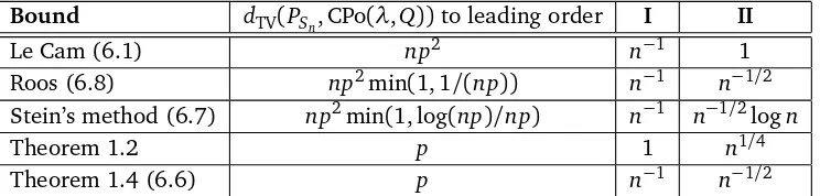
Bound dTV(PSn, CPo(λ,Q))to leading order I II
Le Cam (6.1) np2 n−1 1
Roos (6.8) np2min(1, 1/(np)) n−1 n−1/2
Stein’s method (6.7) np2min(1, log(np)/np) n−1 n−1/2logn
Theorem 1.2 p 1 n1/4
Theorem 1.4 (6.6) p n−1 n−1/2
Table 1: Comparison of the first-order asymptotic performance of the bounds in (6.1), (6.7) and (6.8), with those of Theorems 1.2 and 1.4 for comparable but non-equalQi, in the two
lim-iting regimesp≍1/nandp≍1/pn.
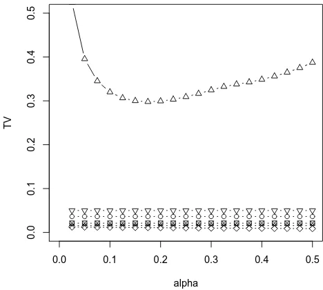
6.2
Example. Compound binomial with equal geometrics
We now examine the finite-nbehavior of the approximation bounds (6.1) – (6.3) in the particular case of equal pi and equal Qi, when Qi is geometric with parameter α > 0, Q(j) = (1−α)αj−1,
j≥1.
Ifα < 12, then{jQ(j)} is decreasing and, withδ= [λ(1−3α+2α2)]−1, the Stein factor in (6.6) becomes
H(λ,Q) =min{1,
p
δ(2−pδ)}. The resulting bounds are plotted in Figures 1 – 3.
6.3
Example. Sums with unequal geometrics
Here, we consider finite-nbehavior of the approximation bounds (6.1), (6.7) and (6.8) in the par-ticular case when the distributionsQi are geometric with parametersαi>0. The resulting bounds
0.0 0.1 0.2 0.3 0.4 0.5
0.0
0.1
0.2
0.3
0.4
0.5
alpha
TV
Figure 1: Bounds on the total variation distance dTV(CQBin(p,Q), CPo(λ,Q)) for Q ∼ Geom(α),
0 50 100 150 200
0.0
0.1
0.2
0.3
0.4
0.5
n
TV
Figure 2: Bounds on the total variation distancedTV(CQBin(p,Q), CPo(λ,Q)) forQ ∼Geom(α)as
in Figure 1, here plotted against the parametern, withα=0.2 andλ=5 fixed.
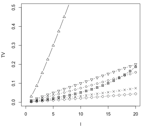
0 5 10 15 20
0.0
0.1
0.2
0.3
0.4
0.5
l
TV
Figure 3: Bounds on the total variation distancedTV(CQBin(p,Q), CPo(λ,Q)) forQ ∼Geom(α)as
In this case, it is clear that the best bounds by a considerable margin are those of Roos[33]given in (6.8).
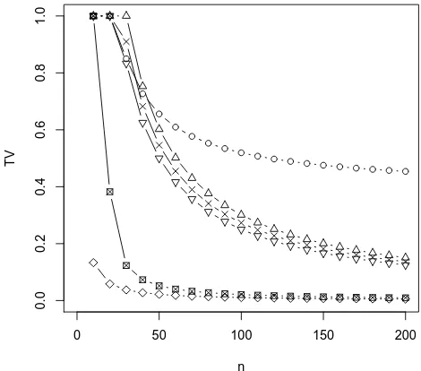
0 50 100 150 200
0.0
0.2
0.4
0.6
0.8
1.0
n
TV
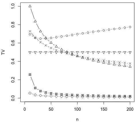
Figure 4: Bounds on the total variation distancedTV(PS
n, CPo(λ,Q))forQi ∼Geom(αi), whereαi
are uniformly spread between 0.15 and 0.25, nvaries, and p is as in regime I, p = 5/n. Again, bounds based onJQ,1are plotted as◦; those based onJQ,2as△; Le Cam’s bound in (6.1) as▽; the
Stein’s method bound in (6.7) as×, and Roos’ bound from Theorem 2 of[33]as⊠. The true total
variation distances, computed numerically in each case, are plotted as⋄.
References
[1] D. Aldous Probability approximations via the Poisson clumping heuristic. Springer-Verlag, New York, 1989. MR0969362
[2] S. Artstein, K. M. Ball, F. Barthe, and A. Naor. On the rate of convergence in the entropic central limit theorem. Probab. Theory Related Fields, 129(3):381–390, 2004. MR2128238
[3] S. Artstein, K. M. Ball, F. Barthe, and A. Naor. Solution of Shannon’s problem on the mono-tonicity of entropy. J. Amer. Math. Soc., 17(4):975–982 (electronic), 2004. MR2083473
[4] A. D. Barbour and L. H. Y. Chen.Stein’s method and applications.Lecture Notes Series. Institute for Mathematical Sciences. National University of Singapore,5, Published jointly by Singapore University Press, Singapore, 2005. MR2201882
0 50 100 150 200
0.0
0.2
0.4
0.6
0.8
1.0
n
TV
Figure 5: Bounds on the total variation distancedTV(PS
n, CPo(λ,Q)) forQi ∼Geom(αi)as in
Fig-ure 4, where αi are uniformly spread between 0.15 and 0.25, nvaries, and p is as in Regime II, p=p0.5/n.
[6] A. D. Barbour and O. Chryssaphinou. Compound Poisson approximation: a user’s guide. Ann. Appl. Probab., 11(3):964–1002, 2001. MR1865030
[7] A. Barbour, L. Holst, and S. Janson. Poisson Approximation. The Clarendon Press Oxford University Press, New York, 1992. MR1163825
[8] A. Barron. Entropy and the central limit theorem. Ann. Probab., 14:336–342, 1986. MR0815975
[9] S. Bobkov and M. Ledoux. On modified logarithmic Sobolev inequalities for Bernoulli and Poisson measures. J. Funct. Anal., 156(2):347–365, 1998. MR1636948
[10] I.S. Borisov, and I.S. Vorozhe˘ıkin. Accuracy of approximation in the Poisson theorem in terms ofχ2distance. Sibirsk. Mat. Zh., 49(1):8–22, 2008. MR2400567
[11] V. ˇCekanaviˇcius and B. Roos. An expansion in the exponent for compound binomial approxi-mations. Liet. Mat. Rink., 46(1):67–110, 2006. MR2251442
[12] T. Cover and J. Thomas.Elements of Information Theory. J. Wiley, New York, 1991. MR1122806
[14] P. Diaconis and S. Holmes. Stein’s method: expository lectures and applications. Institute of Mathematical Statistics Lecture Notes—Monograph Series, 46. Beachwood, OH, 2004. MR2118599
[15] T. Erhardsson. Stein’s method for Poisson and compound Poisson approximation. In A. D. Barbour and L. H. Y. Chen, editors,An Introduction to Stein’s Method, volume 4 ofIMS Lecture Note Series, pages 59–111. Singapore University Press, 2005. MR2235449
[16] P. Harremoës. Binomial and Poisson distributions as maximum entropy distributions. IEEE Trans. Inform. Theory, 47(5):2039–2041, 2001. MR1842536
[17] O. Johnson. Information theory and the central limit theorem. Imperial College Press, London, 2004. MR2109042
[18] O. Johnson. Log-concavity and the maximum entropy property of the Poisson distribution.
Stochastic Processes and Their Applications, 117(6):791–802, 2007. MR2327839
[19] O. Johnson and A. Barron. Fisher information inequalities and the central limit theorem.
Probab. Theory Related Fields, 129(3):391–409, 2004. MR2128239
[20] O. Johnson, I. Kontoyiannis, and M. Madiman, Log-concavity, ultra-log-concavity and a maxi-mum entropy property of discrete compound Poisson measures.Preprint, October 2009. Earlier version online atarXiv:0805.4112v1, May 2008.
[21] I. Johnstone and B. MacGibbon. Une mesure d’information caractérisant la loi de Poisson. In
Séminaire de Probabilités, XXI, pages 563–573. Springer, Berlin, 1987. MR0942005
[22] A. Kagan. A discrete version of the Stam inequality and a characterization of the Poisson distribution. J. Statist. Plann. Inference, 92(1-2):7–12, 2001. MR1809692
[23] I. Kontoyiannis, P. Harremoës, and O. Johnson. Entropy and the law of small numbers. IEEE Trans. Inform. Theory, 51(2):466–472, February 2005. MR2236061
[24] I. Kontoyiannis and M. Madiman. Measure concentration for Compound Poisson distributions.
Elect. Comm. Probab., 11:45–57, 2006. MR2219345
[25] L. Le Cam. An approximation theorem for the Poisson binomial distribution. Pacific J. Math., 10:1181–1197, 1960. MR0142174
[26] L. Le Cam. On the distribution of sums of independent random variables. In Proc. Internat. Res. Sem., Statist. Lab., Univ. California, Berkeley, Calif., pages 179–202. Springer-Verlag, New York, 1965. MR0199871
[27] M. Madiman. Topics in Information Theory, Probability and Statistics. PhD thesis, Brown Uni-versity, Providence RI, August 2005. MR2624419
[28] M. Madiman and A. Barron. Generalized entropy power inequalities and monotonicity prop-erties of information. IEEE Trans. Inform. Theory, 53(7), 2317–2329, July 2007. MR2319376
[30] R. Michel. An improved error bound for the compound Poisson approximation of a nearly homogeneous portfolio. ASTIN Bull., 17:165–169, 1987.
[31] M. Romanowska. A note on the upper bound for the distrance in total variation between the bi-nomial and the Poisson distribution.Statistica Neerlandica, 31(3):127–130, 1977. MR0467889
[32] B. Roos. Sharp constants in the Poisson approximation. Statist. Probab. Lett., 52:155–168, 2001. MR1841404
[33] B. Roos. Kerstan’s method for compound Poisson approximation. Ann. Probab., 31(4):1754– 1771, 2003. MR2016599
[34] F. Topsøe. Maximum entropy versus minimum risk and applications to some classical discrete distributions. IEEE Trans. Inform. Theory, 48(8):2368–2376, 2002. MR1930296
[35] A. M. Tulino and S. Verdú. Monotonic decrease of the non-Gaussianness of the sum of in-dependent random variables: A simple proof. IEEE Trans. Inform. Theory, 52(9):4295–4297, September 2006. MR2298559
[36] W. Vervaat. Upper bounds for the distance in total variation between the binomial or negative binomial and the Poisson distribution. Statistica Neerlandica, 23:79–86, 1969. MR0242235
[37] L. Wu. A new modified logarithmic Sobolev inequality for Poisson point processes and several applications. Probab. Theory Related Fields, 118(3):427-438, 2000. MR1800540