COMBINATORIAL PROPERTIES OF FOURIER-MOTZKIN ELIMINATION∗
GEIR DAHL†
Abstract. Fourier-Motzkin elimination is a classical method for solving linear inequalities in
which one variable is eliminated in each iteration. This method is considered here as a matrix operation and properties of this operation are established. In particular, the focus is on situations where this matrix operation preserves combinatorial matrices (defined here as (0,1,−1)-matrices).
Key words. Linear inequalities, Fourier-Motzkin elimination, Network matrices.
AMS subject classifications.05C50, 15A39, 90C27.
1. Introduction. Fourier-Motzkin elimination is a computational method that may be seen as a generalization of Gaussian elimination. The method is used for finding one, or even all, solutions to a given linear system of inequalities
Ax≤b
whereA∈Rm,n andb∈Rm. Here vector inequality is to be interpreted component-wise. The solution set of the system Ax≤b is a polyhedron which we denote byP, i.e., P ={x∈Rn :Ax≤b}. The method also finds the projection ofP into certain coordinate subspaces. The idea is to eliminate one variable at the time and rewrite the system accordingly (see Section 2). The method was introduced by Fourier in 1827 [3] and his work was motivated by problems in mechanics, least squares etc. A more systematic study of the method was given in Dines [2]. The method was de-scribed in the Ph.D. thesis of T.S. Motzkin [5] and the connection to polyhedra was investigated. Kuhn [4] also described the method and used it to give a proof of Farkas’ lemma. A presentation of Fourier-Motzkin elimination and its role in computations involving polyhedra (for conversions between different representations of polyhedra) is found in Ziegler [8]. For historical notes and references on linear inequalities and Fourier-Motzkin elimination we refer to Schrijver [7].
In this paper we view Fourier-Motzkin elimination as a matrix operation that transforms the given coefficient matrix into a newone, and our goal is to investigate this operation. The focus is on combinatorial aspects of the operation. This casts light on the operation of projection of polyhedra into coordinate subspaces. In Section 2 Fourier-Motzkin elimination is described and in Section 3 we introduce the mentioned matrix operation, denoted the F M operation. This operation is investigated for incidence matrices in Section 4 and for network matrices and related matrices in Section 5.
We nowdescribe some of the notation used in this paper. IfAandBare matrices of the same size, thenA≥B means that the inequality holds componentwise. An all
∗Received by the editors 10 March 2005. Accepted for publication 23 September 2007. Handling
Editor: Bryan L. Shader.
†Centre of Mathematics for Applications, and Dept. of Informatics, University of Oslo, P.O. Box
zeros matrix (of suitable size) is denoted byO. If A ∈Rm,n and I ⊆ {1,2, . . . , m} and J ⊆ {1,2, . . . , n}, then A(I, J) is the submatrix of A formed by the rows in I and columns inJ. IfI={1,2, . . . , m}w e simply w riteA(:, J). The jth column ofA is denoted by A(:, j). The transpose of a matrix Ais denoted by AT. Thejth unit vector (inRn) is denoted byej.
2. Fourier-Motzkin elimination. We briefly reviewthe Fourier-Motzkin elim-ination method. Consider again a linear systemAx≤bwhereA∈Rm,n,b∈Rmand letI:={1,2, . . . , m}. We write the system in component form
a11x1 + a12x2 + · · · + a1nxn ≤b1
a21x1 + a22x2 + · · · + a2nxn ≤b2
.. .
am1x1 + am2x2 + · · · + amnxn ≤bm.
(2.1)
Say that we want to eliminatex1 from the system (2.1). For each i where ai1 = 0
we multiply the i’th inequalityn
j=1aijxj ≤bi by 1/|ai1|. This gives an equivalent
system
x1 + a′i2x2 + · · · + a′inxn ≤b′i (i∈I+)
ai2x2 + · · · + ainxn ≤bi (i∈I0)
−x1 + a′i2x2 + · · · + a′inxn ≤b′i (i∈I−) (2.2)
whereI+ ={i:ai
1>0},I0 ={i:ai1= 0},I− ={i:ai1<0},a′ij =aij/|ai1|and
b′
i=bi/|ai1|. Thus, the rowindex setI={1,2, . . . , m}is partitioned into subsetsI+, I0 andI−, some of which may be empty. It follows thatx
1, x2, . . . , xn is a solution
of the original system (2.1) if and only ifx2, x3, . . . , xn satisfy
n
j=2a′kjxj−b′k ≤b′i−
n
j=2a′ijxj (i∈I+, k∈I−)
n
j=2aijxj ≤bi (i∈I0)
(2.3)
andx1 satisfies
max k∈I− (
n
j=2
a′kjxj−b′k)≤x1≤min
i∈I+(b ′ i−
n
j=2
a′ijxj). (2.4)
If I−(resp. I+) is empty, the first set of constraints in (2.3) vanishes and the
maximum (resp. minimum) in (2.4) is interpreted as∞ (resp. −∞). IfI0 is empty
and eitherI− orI+ is empty too, then we terminate: the general solution ofAx≤b is obtained by choosingx2, x3, . . . , xn arbitrarily and choosingx1 according to (2.4).
The constraint in (2.4) says thatx1 lies in a certain interval which is determined
byx2, x3, . . . , xn. The polyhedron defined by (2.3) is the projection of P along the
x1-axis, i.e., into the space of the variables x2, x3, . . . , xn. One may then proceed
If l > u one concludes that Ax ≤ b has no solution, otherwise one may choose xn ∈[l, u], and then choosexn−1 in an interval which depends onxn etc. This back
substitution procedure produces a solutionx= (x1, x2, . . . , xn) toAx≤b. Moreover,
everysolution ofAx≤bmay be produced in this way. (If the system is inconsistent, this might possibly be discovered at an early stage and one terminates.)
The number of constraints may growexponentially fast as variables are eliminated using Fourier-Motzkin elimination. Actually, a main problem in practice is that the number of inequalities becomes “too large” during the elimination process, even when redundant inequalities are removed. It is therefore of interest to knowsituations where the projected linear systems are not very large or, at least, have some interesting structure. These questions are discussed in the remaining part of the paper. We refer to [7] and [8] for a further discussion of Fourier-Motzkin elimination and a collection of references on this method.
3. TheF M operation. Fourier-Motzkin elimination is a process that works on linear systems (of inequalities). However, it may also be viewed as an operation on matrices from which a given coefficient matrixAproduces another matrixB.
Consider again a linear system (2.1) and its coefficient matrixA∈Rm,n. LetBbe the coefficient matrix of the newlinear system (2.3), still viewed as a system in all the variablesx1, x2, . . . , xn. B is a realm′×nmatrix withm′=|I+| · |I−|+|I0| ≤m2/4
rows. Thus, using the notation introduced in the previous section, B has a row (0, ai2, ai3, . . . , ain) for eachi∈I0 and a row(0, a′i2+a′k2, a′i3+a′k3, . . . , a′in+a′kn) for each pairi, kwithi∈I+, k∈I−. Such a rowis simply the vector sumA′(i,:)+A′(k,:) whereA′ is the coefficient matrix of the system (2.2). If the first column ofAcontains only positive entries, or only negative entries, or ifAhas no rows, thenBbecomes an empty matrix (no rows). This gives rise to a mapping, denoted byF M, which maps AintoB, i.e.,
B=F M(A).
We also get the mappingF M0which mapsAinto the matrixB0=B(:,{2,3, . . . , n}),
i.e., B0 is obtained fromB by deleting the first column (which is the zero vector).
Thus, B0 is the coefficient matrix of the newlinear system (2.3) in the variables
x2, x3, . . . , xn.
To be mathematically concise, we should considerF M andF M0as mappings on
the equivalence classes of matrices under rowpermutations. Permutations of the rows ofA or B do not play any role here; this is motivated by the fact that permutation of the inequalities of the underlying linear systems does not change the solution set.
Remark 3.1. Assume that A ≥O and letB =F M(A). Then B is obtained
fromAby simply deleting the rows inAcorresponding to positive entries in the first column. Moreover, in (2.4) one only gets an upper bound on the variable x1. A
similar observation holds for nonpositive matrices (and one only gets a lower bound onx1).
The resulting matrix is [B b′] w hereB =F M
0(A) and where Bx≤b′ is the linear
system (2.3).
TheF M andF M0operations may be iterated several times.
Definition 3.2. The matrix operationsF M0k andF Mk are defined by
F M00(A) =F M0(A) =A
and fork= 1,2, . . . , n−1
F Mk
0(A) =F M0(F M0k−1(A))
F Mk(A) =
Ok F Mk
0(A)
whereOk denotes a zero matrix withkcolumns.
Thus,F Mk
0 is the coefficient matrix of the projected linear system obtained from
Ax≤bafter eliminating variablesx1, x2, . . . , xk. The matrixF Mk(A) hasncolumns
whileF Mk
0(A) hasn−kcolumns.
We shall focus on theF M operation for matrices with all entries being 0,−1 or 1; such matrices will be calledcombinatorial matrices. These matrices frequently arise in applications, and the corresponding linear systems consist of linear inequalities of the form
j∈Si
xj ≤bi+ j∈Ti
xj
whereSi andTiare disjoint index sets in{1,2, . . . , n}. In some applications, one may be looking for integral or (0,1)-vectors satisfying such combinatorial inequalities. This is a frequent theme in the area of polyhedral combinatorics.
Definition 3.3. A matrixAis calledFM-combinatorialifF Mk(A) is combina-torial fork= 0,1,2, . . . , n−1.
By Remark 3.1 it is clear that a combinatorial matrixAwith entrywise positive or negative first column is trivially FM-combinatorial (sinceF M(A) is empty).
The following result is an immediate consequence of Definition 3.3 and the men-tioned projection property associated with Fourier-Motzkin elimination.
Proposition 3.4. IfAisF M-combinatorial andbis integral, then the projection
of the polyhedron {x∈ Rn :Ax≤b} into the space of the variables xt, xt
+1, . . . , xn
is defined by linear inequalities with(0,1,−1)-coefficients and integral right-hand-side (1≤t≤n).
The converse of the statement in Proposition 3.4 may not hold; the reason is that Fourier-Motzkin elimination may produce redundant inequalities with coefficients different from 0,±1. Note also that every (0,1)-matrix and every (0,−1)-matrix is trivially F M-combinatorial; this follows from Remark 3.1. Thus, interesting F M -combinatorial matrices contain both positive and negative entries.
The obvious way of checking whether a given matrix Ais F M-combinatorial is to use Fourier-Motzkin elimination and calculateF Mk(A) (1≤k≤n−1).
Example 3.5. Let
A=
1 0 0
−1 −1 1
0 1 1
.
Then
F M0(A) = −1 11 1
and F M02(A) = [2].
SoAis notF M-combinatorial.
The following result is easy to establish directly from the definition of a F M -combinatorial matrix.
Proposition 3.6. The set of F M-combinatorial matrices is closed under the
following operations
• deletion of rows
• duplication of rows
• appending a row of zeros.
Example 3.7. Consider the matrices
A1=
−1 1 1
−1 −1 1
−1 0 0
, A2=
−1 1 1
−1 −1 1
1 0 0
.
A1 is (trivially) F M-combinatorial while A2 is notF M-combinatorial. This shows
that the set of F M-combinatorial matrices is not closed under any of the following operations: (i) multiplying a rowby−1, (ii) appending a rowwhich is a unit vector, (iii) appending a row which is the negative of some existing row, (iv) deleting a column.
Moreover, the set ofF M-combinatorial matrices is not closed under column per-mutations.
4. Incidence matrices. Consider a digraphD= (V, E) with vertex setV and arc setE. For notational simplicity we assume thatV ={1,2, . . . , m}. LetA be the incidence matrixof D. The row s (columns) ofAcorrespond to the vertices (arcs) of D: the column corresponding to the arc (i, j) has a 1 in row i, a−1 in rowj, and zeros in the remaining rows. Fori∈V we defineδ+(i) (δ−(i)) as the set of arcs in E that leaves (enters) vertexi. More generally,δ+(S) (δ−(S)) is the set of arcs (i, j) wherei∈Sandj∈S(i∈S,j∈S). A basic operation in a digraph iscontractionof an arc: it creates a newgraph by deleting an arc (and its parallel arcs) and identifying the two end vertices of that arc. We letχSdenote the incidence vector of a setS⊆E, soχS
e = 1 ife∈S and χSe = 0 otherw ise.
The following theorem says that theF M operation on an incidence matrix cor-responds to contraction in the digraph.
Theorem 4.1. Let Abe the incidence matrix of a digraphD and letebe the arc
corresponding to the first column of A. Let B =F M(A). Then every column of B corresponding toeor its parallel arcs is the zero vector, and the submatrix consisting of the remaining columns ofB is the incidence matrix of the digraphD′obtained from D by contracting e.
Proof. The row s of A correspond to the vertex setV: the rowcorresponding to vertexkisχδ+
(k)−χδ−(k)
. Lete= (i, j) be the arc corresponding to the first column of A. Consider B = F M(A). Each rowinA corresponding to a vertex k ∈ {i, j}
satisfiesak1= 0 and it gives rise to a similar rowof B. The matrixB has only one
more row, and it is obtained by summing the two rows inA corresponding toiand j (asai1= 1 andaj1=−1). This rowbecomes
(χδ+(
i)−χδ−(i)
) + (χδ+(
j)−χδ−(j)
) =χδ+({
i,j})−χδ−({i,j})
and this vector has component zero foreand its parallel arcs. This shows thatB is the incidence matrix of the digraphD′.
A direct consequence of the previous theorem is that incidence matrices form a F M-combinatorial matrix class.
Corollary 4.2. Incidence matrices of directed graphs are F M-combinatorial.
A larger matrix class, containing the incidence matrices, is discussed next. Con-sider a (0,±1)-matrixAof sizem×nwhose row index setImay be partitioned into two setsI1and I2 so that each column equals one of the vectors
1. O,
2. ±ei wherei∈I,
3. ei+ek wherei∈I1,k∈I2,
4. ei−ej wherei, j are distinct and both lie inI1 or inI2.
(4.1)
Let M be the class of all such matrices. It is known that every matrixA ∈ M is totally unimodular (TU), i.e., every minor is−1, 0 or 1, see [1]. One may viewA∈ M
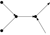
the rows ofAcorrespond to the vertices and the columns to the arcs. There are four types of arcs corresponding to the four column types in (4.1): a zero arc (type 1) with no end vertices, a semi-arc (type 2) with a single end vertex, an undirected arc (type 3) and, finally, a directed arc (type 4). We say that a semi-arc corresponding to the column ei (−ei) leaves (enters) vertex i. Figure 4.1 shows a mixed graph with two directed arcs, two semi-arcs (to the right in the figure) and one undirected arc. (Zero arcs cannot be visualized, but they may be counted.)
Fig. 4.1.A mixed graph.
LetS ⊆I be a vertex subset inD. The operation ofdeletingS from the mixed graphD produces a newmixed graph with vertex set I\S and w ith arcs obtained from those ofDby removing the end vertices inS. Thus, this operation may produce semi-arcs or even zero arcs. The following theorem shows that the incidence matrix of every mixed graph and its transpose both are F M-combinatorial. Moreover, the proof contains a combinatorial interpretation of the elimination of an arc or a vertex as certain operations on the mixed graph.
Theorem 4.3. Let A∈ M. Then bothAandAT are F M-combinatorial. Proof. LetA∈ Mand letB =F M0(A). We showthatB∈ Mby finding a new
mixed graphD′ withB as its incidence matrix. Consider the first column ofA, and its corresponding arce, and distinguish between the four possible cases in (4.1).
1. A(:,1) = O. Then B is the incidence matrix of the mixed graph obtained fromD by deleting the zero arce.
2. A(:,1) =±ei. Then B is the incidence matrix of the mixed graph obtained fromD by deleting the arceand the vertexi.
3. A(:,1) =ei+ek wherei∈I1,k∈I2. ThenB is the incidence matrix of the
mixed graph obtained fromDby deleting the arcethe verticesiandj. 4. A(:,1) =ei−ekwherei, jare distinct and both lie inI1. (The case when both
lie inI2is treated similarly.) ThenB is the incidence matrix ofD′ obtained
from D by deletinge and contracting the verticesi and j into a newsingle vertex. Each arc parallel toe becomes a zero arc and arcs with exactly one vertex amongiandj arc incident to the newvertex (with similar direction). Since bothiand jlie in I1, the matrixB satisfies all properties of (4.1).
Thus,B=F M(A)∈ Mand it follows by induction thatAisF M-combinatorial. Next, considerC=AT whereA∈ Mand letvbe the vertex (of the mixed graph) corresponding to the first column ofC. LetB =F M0(C). ThenB is the incidence
tov. Note that parallel arcs may arise.
undirected arc [v, w] directed arc (v, w) semi-arc leavingv semi-arc enteringv semi-arc leavingw semi-arc enteringw zero arc
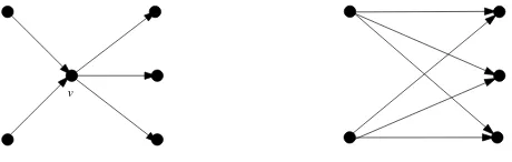
[image:8.612.178.408.268.341.2]directed arc (u, v) new undirected arc[u, w] directed arc(u, w) semi-arc leavingu
Fig. 4.2.New arcs in the elimination ofv.
Again, by induction, it follows thatAT isF M-combinatorial.
In particular, if A is the incidence matrix of a directed graph and we apply Fourier-Motzkin elimination to AT, then elimination of the vertex v corresponds to deleting v and incident arcs from the digraphD and adding an arc (u, w) whenever (u, v) and (v, w) are arcs inD, see Figure 4.3. Thus, F M0(AT) is the transpose of
the incidence matrix of this newdigraph.
v
Fig. 4.3.Elimination ofv.
Corollary 4.4. LetAbe the incidence matrix of a digraphD. Then the matrix
A
−A
isF M-combinatorial.
Proof. Let B =F M(A) soB has the form described in Theorem 4.1. Then we see that
F M( A
−A
) =
B
−B O
where the zero matrix has two rows. The result now follows by induction.
5. Network matrices and extensions. In this section we consider the FM op-eration in connection with network matrices and some related matrices. In particular we are concerned with the role that column permutations play for the FM operation. We refer to Brualdi and Ryser [1] or Schrijver [7] for a discussion of network matrices. Note that every matrix in the classM(see Section 4) is a network matrix.
to an arc e ∈ P+
u,v, a −1 in each column corresponding to an arc e ∈ Pu,v− , and it contains zeros elsewhere. Thus, this row equals χP+
u,v −χPu,v− which we consider as
the signed incidence vector of the pathPu,v.
Consider a pair (D, T) as above and the associated network matrixA. Letv be a leaf ofT (i.e., it has degree 1) and let ebe the incident arc. The digraph obtained from T by deleting v (and e) is denoted by T′ = (V′, E′), so V′ = V \ {v} and E′=E\ {e}. Moreover, define D′ = (V′, F′) w here
F′ = (F\(δD+(v)∪δD−(v)))∪ {(u, w) : (u, v),(v, w)∈F}.
Thus, D′ is obtained from D by deleting v and incident arcs and introducing new arcs of the form (u, w) for each pair (u, v),(v, w)∈F. We say that the pair (T′, D′) is obtained from (D, T) byelimination of v.
Theorem 5.1. Consider a directed tree T = (V, E) and a digraph D = (V, F)
as above with associated network matrix A. Letv be a leaf of T and assume that the incident arc e corresponds to the first column of A. Let (T′, D′) be obtained from (D, T) by elimination of v. Then B = F M0(A) is the network matrix of (T′, D′)
(using the same ordering of arcs inT′ as in T).
Proof. Let as usualD = (V, F). The nonzeros in the first column of A are in those rows corresponding to arcs of the form (u, v) or (v, w) inF. Moreover, the first column contains entries 1 and −1 in a pair of rows that correspond to a pair (u, v), (v, w) w ith (u, v),(v, w) ∈ F. Such a pair gives rise to a row R in B = F M0(A)
which is the sum of the corresponding rows inA. These tw o row s inAare the signed incidence vectors of the two paths Pu,v and Pv,w in the tree T. But then there is a vertex s such that Pu,v = Pu,s ∪Ps,v and Pv,w = Pv,s∪Ps,w; this is due to the fact that T is a tree. It follows that the rowR is the signed incidence vector of the (u, w)-pathPu,s∪Ps,w. The remaining rows of the matrixB are the signed incidence vectors of paths Pu,w where (u, w) ∈ F and u, w =v. Therefore B is the network matrix of (T′, D′).
If we delete a leaf from a treeT we obtain a new tree where we can delete a new leaf etc. until we are left with a single vertex. This induces an ordering of the arcs of T, namely the order in which they are deleted. We call such an ordering of the arcs in T anarc elimination orderingin T. Every nontrivial tree has several arc elimination orderings.
Corollary 5.2. Let A be a network matrix associated with (D, T) where the
columns of A correspond to an arc elimination ordering in the tree T. Then A is F M-combinatorial.
Proof. Since the columns ofAare ordered according to an arc elimination ordering inT, Theorem 5.1 gives thatF M(A) is the network matrix associated with (T′, D′), F M2(A) is the network matrix associated with ((T′)′,(D′)′) etc. So, by induction,A isF M-combinatorial.
The following example illustrates what can happen if the columns of a network matrix do not correspond to an arc elimination ordering inT.
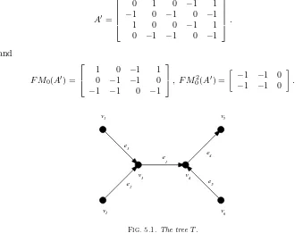
Example 5.3. Consider the treeTin Figure 5.1, and let the arcs inDbe (v1, v6),
arcs inD ordered as above and columns correspond toe1, e2, . . . , e6 (in this order), so A=
1 0 1 0 −1
−1 −1 0 −1 0
1 1 0 0 −1
−1 0 −1 −1 0 . Then
F M0(A) =
−1 1 −1 −1
0 0 −1 −1
0 0 −1 −1
1 −1 −1 −1
and F M02(A) =
0 −2 −2 0 −1 −1 0 −1 −1
.
Let nowA′ be obtained from Aby permuting columns so that the first column inA is the last one inA′. Then
A′ =
0 1 0 −1 1
−1 0 −1 0 −1
1 0 0 −1 1
0 −1 −1 0 −1
. and
F M0(A′) =
1 0 −1 1
0 −1 −1 0
−1 −1 0 −1
, F M02(A′) =
−1 −1 0
[image:10.612.110.449.297.558.2]−1 −1 0 . 1 2 3 4 5 6 2 5 3 4 1 e e e v v v v e e v v
Fig. 5.1.The treeT.
We nowstudy a large class of permuted FM-combinatorial matrices related to network matrices. Consider a partitioned matrixAof the following form
A=
A11 A12 A13 · · · A1p O A22 A23 · · · A2p O O A33 · · · A3p
..
. ... . .. ...
O O · · · App
(5.1)
where (i) all matricesAij are (0,1,−1)-matrices, (ii) the first column inAii is either eor−ewhereeis an all ones vector (i≤p−1), (iii)Aij is arbitrary (1≤i < j≤p), (iv)App is a network matrix. We callB a generalized network matrixif its rows and columns may be permuted to obtain a matrix of the specified from in (5.1), i.e., if A=P BQhas the form (5.1) for suitable permutation matricesP andQ.
The following algorithm may be used to test if a matrix is a generalized network matrix.
Algorithm 1.
Input: a(0,1,−1)-matrixA.
1. Start with the matrixAand perform the following operation recursively: test if the matrix contains a nonnegative or nonpositive column. If so, delete this column and the rows in which it contains its nonzeros.
2. Test if the remaining matrix is a network matrix.
We refer to [6] for a detailed description of an efficient (polynomial time) algorithm for recognizing a network matrix.
Theorem 5.4. Each generalized network matrix is a permuted FM-combinatorial
matrix. Moreover, Algorithm 1 decides in polynomial time whether a given matrixAis a generalized network matrix. The algorithm also finds the desired column permutation that takesA into an FM-combinatorial matrix.
Proof. Assume that B is a generalized network matrix, so A = P BQ has the form (5.1) for suitable permutation matrices P and Q. We may here assume that the columns corresponding to the network matrix App are ordered according to an arc elimination ordering in the associated tree T. We nowapply Fourier-Motzkin elimination to the matrix A. Since the first column of A11 is either e or −e, the
resulting matrixA′ =F M
0(A) is obtained fromAby deleting the first block rowand
the first column. ThenA′ containsk−1 leading columns that are equal to the zero vector, wherekis the number of columns inA11. TheF M0operation simply deletes
thesek−1 zero columns so the resulting matrix is the same as the one obtained from A by deleting the first block rowand the first block column. We proceed similarly with the blockA22, and afterp−1 iterations, we are left with the matrixApp. Then,
by Corollary 5.2, it follows that A is FM-combinatorial. This proves that B is a permuted FM-combinatorial matrix.
Claim: this matrixC isuniquein the sense that it does not depend on the order in which the columns were deleted in Step 1 of the algorithm.
Proof of claim: Consider two possible sequences of column deletions, say π = (π1, π2, . . . , πr) and π′ = (π1′, π2′, . . . , π′s). This means that, in the first (second) sequence, columnπi(π′
i) is deleted in theith step. We prove thatr=sand thatπ′ is a permutation ofπ. Ifπ=π′, we are done. Otherwise, letibe smallest possible such thatπ′
i=πi. This means that, in theith step in theπ′ sequence, it would be feasible to delete column πi, although we decided to delete π′
i instead. This possibility of deleting columnπi (in connection with theπ′ sequence) remains, and therefore there exists a j > i such that π′
j = πi. By iterating this argument we see that π′ must contain all the numbersπi, πi+1, . . . , πr(it is possible to delete these columns in this
order). Similarly, we also see thatπmust contain all the numbersπ′
i, πi′+1, . . . , πs′. It follows thatr=sand thatπ′ is a permutation ofπ.
So, all possible column deletions are permutations of each other. Finally, the set of rows deleted clearly does not depend on the order in which the columns are deleted, but only on which set of columns that is deleted. This shows the uniqueness of C, and the claim follows.
By the claim the matrixC after Step 1 is unique. Moreover,A is a generalized network matrix if and only ifC is a network matrix, and this is determined in Step 2 of the algorithm (using the polynomial time algorithm described in [6]). This proves the theorem.
We nowturn our attention to a class of (0,1,−1)-matrices associated with paths in directed graphs. Apath incidence matrixis a matrix where each row is the signed incidence vector of a path in an underlying fixed digraph D. So each such path consists of an arc sequence connecting the initial vertex to the terminal vertex, and the incidence vector contains a +1 or a−1 for all these arcs where the sign depends on the direction in which the arc is traversed.
Every network matrix is a path incidence matrix (where the underlying digraph D is a tree), and by Corollary 5.2, these matrices are permuted FM-combinatorial. Moreover, it is possible to construct examples of path incidence matrices that arenot permuted FM-combinatorial, see below. This property (permuted FM-combinatorial) seems to reflect a complicated interplay between the selection of paths and the struc-ture of the underlying digraphD.
Our final result characterizes the digraphsDfor whichallpath incidence matrices are permuted FM-combinatorial.
Theorem 5.5. Consider a digraph Dand the corresponding undirected graphG.
Then every path incidence matrix associated withD is permuted FM-combinatorial if and only if Gis acyclic.
Proof. Let A be a path incidence matrix in a digraphD where the correspond-ing undirected graph G is acyclic. Then G decomposes into a set of disjoint trees T1, T2, . . . , Tk. By suitable permutations of the rows and columns of A w e obtain
a matrix which is the direct sum of path incidence matrices corresponding to the treesT1, T2, . . . , Tk. Furthermore, we may order the columns of this matrix according
this permuted matrixA is FM-combinatorial, so the original matrix A is permuted FM-combinatorial.
Assume next thatG(the undirected graph associated with D) contains a cycle. Let e1, e2, . . . , ek be the arcs in this cycle (ordered consecutively). For simplicity of
presentation we assume that all arcs in the cycle have the same direction (so the tail ofei is the head of ei+1 for each i); the general case where the directions vary
can be treated similarly. For each i ≤ k consider the three paths P1
i = (ei−1, ei), P2
i = (ei, ei+1), and Pi3 = (ei−1, ei, ei+1), as well as the three paths that are the
opposite ofP1
i,Pi2 and Pi3 (e.g., the opposite path of Pi1 is (ei, ei−1). LetAbe the
path incidence matrix corresponding to these 6kpaths. This matrix may contain some columns that are equal to the zero vector; they correspond to arcs outsideC. Consider a arbitrary ordering of the columns ofAand apply Fourier-Motzkin elimination based on this ordering. Whenever we meet a column which is the zero vector, that column will simply be deleted. Eventually we come to the first column corresponding to an arc in C, say this is ei. Let B be the matrix obtained after eliminating ei. Then B contains the following submatrix corresponding to the columnsei−1andei+1 and
suitable rows
B∗=
1 −1
1 1
−1 −1
.
The entries in the remaining columns of B in these rows are all zero. Therefore, eventually we have to eliminate either ei−1 or ei+1 and, in either case, we see from
B∗ that we will get an entry which is equal to 2 or−2. This proves that the original matrixAis not permuted FM-combinatorial.
Acknowledgment. The author would like to thank the referee for several valu-able comments. Also, thanks to Kristina R. Dahl for interesting discussions in con-nection with Theorem 5.4.
REFERENCES
[1] R.A. Brualdi and H.J. Ryser. Combinatorial matrix theory. Encyclopedia of Mathematics. Cambridge University Press, Cambridge, 1991.
[2] L.L. Dines. Systems of linear inequalities. The Annals of Mathematics, 2nd Ser., 20 (No. 3): 191–199, 1919.
[3] J.J.-B. Fourier. Oeuvres II. Paris, 1890.
[4] H.W. Kuhn. Solvability and consistency for linear equations and inequalities. The American Mathematical Monthly, 63 (No. 4): 217–232, 1956.
[5] T.S. Motzkin. Beitr¨age zur Theorie der linearen Ungleichungen. Thesis, 1936. Reprinted in:
Theodore S. Motzkin: selected papers(D. Cantor et al., eds.), Birkh¨auser, Boston, 1983. [6] G. Nemhauser and L.A. Wolsey. Integer and combinatorial optimization. Wiley, New York,
1988.