Full Terms & Conditions of access and use can be found at
http://www.tandfonline.com/action/journalInformation?journalCode=ubes20
Download by: [Universitas Maritim Raja Ali Haji] Date: 12 January 2016, At: 17:53
Journal of Business & Economic Statistics
ISSN: 0735-0015 (Print) 1537-2707 (Online) Journal homepage: http://www.tandfonline.com/loi/ubes20
The Identification Power of Equilibrium in Simple
Games
Andres Aradillas-Lopez & Elie Tamer
To cite this article: Andres Aradillas-Lopez & Elie Tamer (2008) The Identification Power of Equilibrium in Simple Games, Journal of Business & Economic Statistics, 26:3, 261-283, DOI: 10.1198/073500108000000105
To link to this article: http://dx.doi.org/10.1198/073500108000000105
Published online: 01 Jan 2012.
Submit your article to this journal
Article views: 278
The Identification Power of Equilibrium
in Simple Games
Andres ARADILLAS-LOPEZ
Department of Economics, Princeton University, Princeton, NJ 08544
Elie TAMER
Department of Economics, Northwestern University, Evanston, IL 60208 (tamer@northwestern.edu)
We examine the identification power that (Nash) equilibrium assumptions play in conducting inference about parameters in some simple games. We focus on three static games in which we drop the Nash equilibrium assumption and instead use rationalizability as the basis for strategic play. The first example examines a bivariate discrete game with complete information of the kind studied in entry models. The second example considers the incomplete-information version of the discrete bivariate game. Finally, the third example considers a first-price auction with independent private values. In each example, we study the inferential question of what can be learned about the parameter of interest using a random sample of observations, under level-krationality, wherekis an integer≥1. Askincreases, our identified set shrinks, limiting to the identified set under full rationality or rationalizability (ask→ ∞). This is related to the concepts of iterated dominance and higher-order beliefs, which are incorporated into the econometric analysis in our framework. We are then able to categorize what can be learned about the parameters in a model under various maintained levels of rationality, highlighting the roles of different assumptions. We provide constructive identification results that lead naturally to consistent estimators.
KEY WORDS: Equilibrium vs rationality; Identification; Partial identification.
1. INTRODUCTION
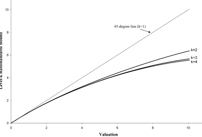
In this article we examine the identification power of equilib-rium in some simple games. In particular, we relax the assump-tion of Nash equilibrium (NE) behavior and assume that players are rational. Rationality posits that agents play strategies that are consistent with a set of proper beliefs. The object of interest in these games is a parameter vector that parameterizes payoff functions. We study the identified features of the model using a random sample of data under a set of rationality assumptions, culminating with rationalizability, a concept introduced jointly in the literature by Bernheim (1984) and Pearce (1984), and compare those to what we can learn under Nash. We find that in static discrete games withcomplete information, the identified features of the games with more than one level of rationality are similar to those obtained with Nash behavior assumption but allowing for multiple equilibria (including equilibria in mixed strategies). In a bivariate game withincomplete information, if the game has a unique (Bayesian) NE, then there is convergence between the identified features with and without equilibrium only when the level of rationality tends to infinity. When there are multiple equilibria, the identified features of the game under rationality and equilibrium are different: smaller identified sets (hence more information about the parameter of interest) when equilibrium is imposed, but computationally easier to construct identification regions under rationality (i.e., no need to solve for fixed points). In the auction game that we study, the situ-ation is different. We follow the work of Battigalli and Sinis-chalchi (2003) where, under some assumptions given the valu-ations, rationalizability predicts only upper bounds on the bids. We show how these bounds can be used to learn about learn about the latent distribution of valuation. Another strategic as-sumptions in auctions resulting in tighter bounds is the concept
ofP-dominance studied by Dekel and Wolinsky (2003).
Economists have observed that equilibrium play in noncoop-erative strategic environment is not necessary for rational be-havior. Some can easily construct games in which NE strategy
profiles are unreasonable, whereas others can find reasonable strategy profiles that are not Nash. Restrictions once Nash be-havior is dropped typically are based on a set of “rationality” criteria, as has been enumerated in numerous works under dif-ferent strategic scenarios. In this article we study the effect of adopting a particular rationality criterion on learning about pa-rameters of interests. We do not advocate one type of strategic assumption over another, but simply explore one alternative to Nash and evaluate its effect on parameter inference. Thus, de-pending on the application, identification of parameters of in-terest certainly can be studied under strategic assumptions other than rationalizability. We provide such an example.
Because every Nash profile is rational under our definition, dropping equilibrium play complicates the identification prob-lem, because under rationality only, the set of predictions is enlarged. As Pearce noted, “this indeterminacy is an accurate reflection of the difficult situation faced by players in a game, because logical guidelines and the rules of the game are not sufficient for uniqueness of predicted behavior.” Thus it is in-teresting from the econometric perspective to examine how the identified features of a particular game changes as weaker as-sumptions on behavior are made.
We maintain that players in the game are rational, where heuristically, we define rationality as behavior consistent with an optimizing agent equipped with a proper set of beliefs or probability distributions about the unknown actions of others. Rationality comes in different levels or orders, where a profile is first-order rational if it is a best response to some profile for the other players. This intersection of layers of rationality consti-tutes rationalizable strategies. We study the identification ques-tion for level-krationality fork≥1. When we study the identi-fying power of a game under a certain set of assumptions on the
© 2008 American Statistical Association Journal of Business & Economic Statistics July 2008, Vol. 26, No. 3 DOI 10.1198/073500108000000105
261
strategic environment, we implicitly assume that all players in that game are abiding exactly by these assumptions and playing exactly that game. This is important, because theoretical work has challenged the multiplicity issues that arise under rational-izability. For example, Weinstein and Yildiz (2007) showed that for any rationalizable set of strategies in a given game, there is a local disturbance of that game in which these are the unique rationalizable strategies. This ambiguity about what is the exact game being played is why it is important to study the identified features of a model in the presence of multiplicity.
Using equilibrium as a restriction to gain identifying power is a well-known strategy in economics. The model of demand and supply uses equilibrium to equate the quantity demanded with quantity supplied, thus obtaining the classic simultaneous equa-tion model. Other literature in econometrics, such as job search models and hedonic equilibrium models, explicitly use equi-librium as a “moment condition.” In this article we study the identification question in simple game-theoretic models with-out the assumption of equilibrium by focusing on the weaker concept of rationality,k-level rationality and its limit rational-izability. This approach has two important advantages. First, it leads naturally to a well-defined concept oflevels of rational-ity, which is attractive practically. Second, it can be adapted to a very wide class of models without the need to introduce ad hoc assumptions. Ultimately, interim rationalizability allows us to do inference (to varying degrees) both on the structural pa-rameters of a model (e.g., the payoff papa-rameters in a reduced-form game or the distribution of valuations in an auction) and on the properties ofhigher-order beliefsby the agents, which are incorporated into the econometric analysis. The features of this hierarchy of beliefs characterize what we call the rational-ity level of agents. In addition, it is possible to also provide testable restrictions that can be used to find an upper bound on the rationality level in a given data set.
Level-kthinking as an alternative to Nash equilibrium be-havior also has been studied by Stahl and Wilson (1995), Nagel (1995), Ho, Camerer, and Weigelt (1998), Costa-Gomes, Craw-ford, and Broseta (2001), Costa-Gomes and Crawford (2006), and Crawford and Iriberri (2007). These models depart from equilibrium behavior by dropping the assumption that each player has a perfect model of others’ decisions and replacing
it with the assumption that such subjective models survive k
rounds of iterated elimination of dominated decisions. Thus each player’s subjective model about others’ behavior is consis-tent with level-kinterim rationalizability in the sense of Bern-heim (1984). For identification, the aforementioned articles as-sume the existence of a small number of prespecified types, each of which is associated with a very specific behavior. For example, a particular type of player could perform two mental rounds of deletion of dominated strategies and best response to a uniform distribution over the surviving actions. Using care-fully designed experiments, previous researchers sought to ex-plain which type best fits the observed choices. This article dif-fers from the aforementioned works by focusing on bounds for conditional choice probabilities that can be rationalized by be-liefs that survive ksteps of iterated thinking. We look at the largest possible set of level-krationalizable beliefs but assume nothing about how players choose their actual (unobserved) be-liefs from within this set. In addition, we focus on situations in
which the researcher ignores how “rational” players are and in which other primitives of the game also are the object of inter-est: payoff parameters in discrete games or the distribution of valuations in an auction. In an experimental data set, the last set of objects are entirely under the control of the researcher, and strong parametric assumptions typically are made about behav-ioral types.
In Section 2 we review and define rational play in a nonco-operative strategic game. Here we mainly adapt the definition provided by Pearce. We then examine the identification power of dropping Nash behavior in some commonly studied games in empirical economics. In Section 3 we consider discrete static games of complete information. This type of game is widely used in the empirical literature on (static) entry games with complete information and under NE (see, e.g., Bjorn and Vuong 1985; Bresnahan and Reiss 1991; Berry 1994; Tamer 2003; An-drews, Berry, and Jia 2003; Ciliberto and Tamer 2003; Bajari,
Hong, and Ryan 2005). Here we find that in the 2×2 game
with level-2 rationality, the outcomes of the game coincide with Nash, and thus econometric restrictions are the same. In Sec-tion 4 we consider static games with incomplete informaSec-tion. Empirical frameworks for these games have been studied by Aradillas-Lopez (2005), Aguiregabiria and Mira (2007), Seim (2002), Pakes, Porter, Ho, and Ishii (2005), Berry and Tamer (1996), and others. Characterization of rationalizability in the incomplete information game is closely related to the higher-order belief analysis in the global games literature (see Morris and Shin 2003) and to other recently developed concepts, such as those of Dekel, Fudenberg, and Morris (2007) and Dekel, Fu-denberg, and Levine (2004). Here we show that level-k rational-ity implies restrictions on player beliefs in the 2×2 game that lead to simple restrictions that can be exploited in identification. Askincreases, an iterative elimination procedure restricts the size of the allowable beliefs that map into stronger restrictions that can be used for identification. If the game admits a unique equilibrium, then the restrictions of the model converge toward Nash restrictions as the level of rationality k increases. With multiple equilibria, the iterative procedure converges to sets of beliefs that contain both the “large” and ”small” equilibria. In particular, studying identification in these settings is simple, be-cause we do not need to solve for fixed points, but simply iterate the beliefs toward the predetermined level of rationalityk. In Section 5 we examine a first-price independent auction game, where we follow the work of Battigalli and Sinischalchi (2003). Here for any orderk, we are only able to bound the unobserved valuation from above. Finally, in Section 6 we conclude.
2. NASH EQUILIBRIUM AND RATIONALITY
In noncooperative strategic environments, optimizing agents maximize a utility function that depends on what their oppo-nents do. In simultaneous games, agents attempt to predict what their opponents will play, and then play accordingly. Nash be-havior posits that players’ expectations of what others are doing are mutually consistent, and so a strategy profile is Nash if no player has an incentive to change strategy given what the other agents are playing. This Nash behavior makes an implicit as-sumption on players’ expectations. But, players “are not com-pelled by deductive logic” (Bernheim) to play Nash. In this
article we examine the effect of assuming Nash behavior on identification by comparing restrictions under Nash with those obtained under rationality in the sense of Bernheim and Pearce. Here we follow Pearce’s framework and first maintain the fol-lowing assumptions on behavior:
• Players use proper subjective probability distribution, or use the axioms of Savage, when analyzing uncertain events.
• Players are expected utility maximizers.
• Rules and structure of the game are common knowledge.
We next describe heuristically what is meant by rationalizable strategies; precise definitions have been given by Pearce (1984), for example:
• We say that a strategy profile for playeri(which can be a mixed strategy) isdominatedif there exists another strat-egy for that player that does better no matter what other agents are playing.
• Given a profile of strategies for all players, a strategy for playeri is abest responseif that strategy does better for that player than any other strategy given that profile.
To define rationality, we use the following notation. LetRi(0)
be the set of all (possibly mixed) strategies that playerican play andR−i(0)be the set of all strategies for players other thani.
Then, heuristically, we have the following:
• Level-1 rational strategiesfor playeriare strategy profiles
si∈Ri(0)such that there exists a strategy profile for other
players inR−i(0)for whichsi is a best response. The set
of level-1 strategies for playeriisRi(1).
• Level-2 rational strategiesfor playeriare strategy profiles
si∈Ri(0)such that there exists a strategy profile for other
players inR−i(1)for whichsiis a best response.
• Level-t rational strategies are defined recursively from level 1.
Note that by construction, Ri(t)⊆Ri(t−1). Finally, ratio-nalizable strategiesare ones that lie in the intersection of the
R’s astincreases to infinity. In the complete information game
of Section 3, we show that there exists a finiteksuch that for
Ri(t)=Ri(k)for allt≥k. In the incomplete information
mod-els of Sections 4 and 5, we show that we can haveRi(t)⊂Ri(k)
for allt>k. In all of these settings, a strategy is level-krational for a player if it is a best response to some strategy profile in
Ri(k−1)by his opponents. Iterating this further, we arrive at
the set of rationalizable strategies. Pearce provided properties of the rationalizable set; for example, NE profiles are always included in this set, and the set contains at least one profile in pure strategies.
3. BIVARIATE DISCRETE GAME WITH COMPLETE INFORMATION
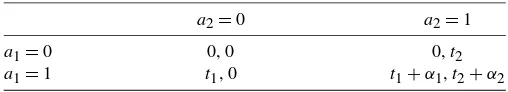
Consider the following bivariate discrete 0/1 game wheretp
is the payoff that playerpobtains by playing 1 when player−p
is playing 0. Parametersα1andα2are of interest. The
econo-metrician does not observet1ort2and is interested in learning
about theα’s and the joint distribution of(t1,t2). (See Table 1.)
Assume also, as in entry games, that theα’s are negative. In this
Table 1. Bivariate discrete game
a2=0 a2=1
a1=0 0, 0 0,t2
a1=1 t1, 0 t1+α1,t2+α2
example and the next, we assume that we have access to a ran-dom sample of observations (y1i,y2i)Ni=1, which represent, for
example, market structures in a set ofNindependent markets.
To learn about the parameters, we map the observed distrib-ution of the data (the choice probabilities) to the distribdistrib-ution predicted by the model. Because this is a game of complete information, players observe all of the payoff-relevant informa-tion. In particular, in the first round of rationality, player 1 will play 1 ift1+α1≥0, because this will be a dominant strategy.
In addition, ift1is negative, then player 1 will play 0. But when t1+α1≤0≤t1, both actions 1 and 0 are level-1 rational;
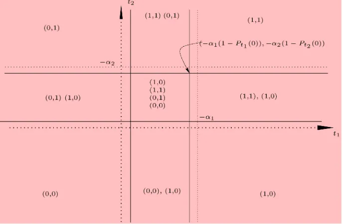
ac-tion 1 is raac-tional because it can be a best response to player 2 playing 0, whereas action 0 is a best response to player 2 play-ing 1. The setR(1)is summarized in Figure 1. Consider, for ex-ample the upper right corner. For values oft1andt2lying there,
playing 0 is not a best response for either player. Thus (1,1)
is the unique level-1 rationalizable strategy (which is also the unique NE). Consider now the middle region on the right side, that is,(t1,t2)∈ [−α1,∞)× [0,−α2]. In level-1 rationality, 0
is not a best reply for player 1, but player 2 can play either 1 or 0; 1 is a best reply when player 1 plays 0, and 0 is a best reply for player 2 when player 1 plays 1. However, in the next round of rational play, given that player 2 now believes that player 1 will play 1 with probability 1, then player 2’s response is to play 0. Thus R(1)= {{1},{0,1}} while the rationalizable set
reduces to the outcome(1,0). Here R(k)=R(2)= {{1},{0}}
for allk≥2. In the middle square, we see that the game pro-vides no observable restrictions; any outcome can bepotentially observable, because both strategies are rational at any level of rationality. Note also that in this game, the set of rationalizable strategies is the set of profiles that are undominated. This is a property of bivariate binary games.
3.1 Implications of Level-k Rationality
A random sample of observations allows us to obtain a con-sistent estimator of the choice probabilities (or the data). The object of interest here isθ=(α1, α2,F(·,·)), whereF(·,·)is
the joint distribution of (t1,t2). One interesting approach to
conduct inference on the identified set, I, is to assume that
botht1andt2are discrete random variables with identical
sup-port on s1, . . . ,sK such that P(t1=si;t2=sj)=pij ≥0 for i,j∈ {1, . . . ,k}withi,jpij=1. Thus we make inference on
the set of probabilities(pij,i,j≤k)and(α1, α2). We highlight
this for level-2 rationality. In particular, we say that
θ=((pij), α1, α2)∈I
if and only if
P11=
i,j pij
1[si≥ −α1;sj≥ −α2]
+l(ij1,1)1[0≤si≤ −α1;0≤sj≤ −α2]
,
Figure 1. Rationalizable profiles in a bivariate game with complete information.
P00=
i,j pij
1[si≤0;sj≤0]
+l(ij0,0)1[0≤si≤ −α1;0≤sj≤ −α2]
,
P10=
i,j pij
1[si≥0;sj≤0] +1[si≥ −α1;0≤sj≤ −α2]
+l(ij1,0)1[0≤si≤ −α1;0≤sj≤ −α2]
,
and
P01=
i,j pij
1[si≤0;sj≥0] +1[0≤si≤ −α1;sj≥ −α2]
+l(ij0,1)1[0≤si≤ −α1;0≤sj≤ −α2]
for some (l(ij1,1),lij(0,0),l(ij0,1),l(ij1,0)) ≥0 and lij(1,1) +l(ij0,0) +
lij(0,1)+lij(1,0)=1 for all i,j≤k. The l’s can be thought of as the “selection mechanisms” that choose an outcome in the re-gion where the model predicts multiple outcomes. We treat the support points as known, but this is without loss of
general-ity, because those also can be made part of θ. The foregoing
equalities (and inequalities) for a givenθ are similar to first-order conditions from a linear programming problem and thus can be solved rapidly using linear programming algorithms. In particular, consider the objective function in (1). Note first that
Q(θ )≤0 for allθ’s in the parameter space. Moreover,
θ∈I
if and only ifQ(θ )=0.
Q(θ )= max
vi,...,v8,(l(ij1,1),l
(0,0)
ij ,l
(0,1)
ij ,l
(1,0)
ij )
−(v1+ · · · +v8) s.t.
P11−
i,j pij
1[si≥ −α1;sj≥ −α2]
+l(ij1,1)1[0≤si≤ −α1;0≤sj≤ −α2]
=v1−v2, P00−
i,j pij
1[si≤0;sj≤0]
+l(ij0,0)1[0≤si≤ −α1;0≤sj≤ −α2]
=v3−v4,
P10−
i,j pij
1[si≥0;sj≤0]
(1)
+1[si≥ −α1;0≤sj≤ −α2]
+l(ij1,0)1[0≤si≤ −α1;0≤sj≤ −α2]
=v5−v6,
P01−
i,j pij
1[si≤0;sj≥0] +1[0≤si≤ −α1;sj≥ −α2]
+l(ij0,1)1[0≤si≤ −α1;0≤sj≤ −α2]
=v7−v8, vi≥0;
lij(1,1),lij(0,0),lij(0,1),l(ij1,0)≥0;
lij(1,1)+l(ij0,0)+lij(0,1)+l(ij1,0)=1 for all 1≤i,j≤k.
First, note that for anyθ, the program is feasible; for exam-ple, set(l(ij1,1),lij(0,0),lij(0,1),lij(1,0))=0 and then setv1=P11−
i,jpij1[si≥ −α1;sj≥ −α2]andv2=0 ifP11−i,jpij1[si≥
−α1;sj≥ −α2] ≥0, or set v2= −(P11−i,jpij1[si≥ −α1; sj ≥ −α2]) and v1=0 and similarly for the rest. Moreover,
θ∈Iif and only ifQ(θ )=0. We can collect all of the
parame-ter values for which the foregoing objective function is equal to 0 (or approximately equal to 0). A similar linear programming procedure was used by Honoré and Tamer (2006). The sampling variation comes from having to replace the choice probabilities
(P11,P12,P21,P22)with their sample analogs, which results in
a sample objective functionQn(·)that can be used to conduct
inference.
More generally, and without making support assumptions, a practical way to conduct inference with one level of ratio-nality, say, is to use an implication of the model. In particular, underk=1 rationality, the statistical structure of the model is one of moment inequalities,
Pr(t1≥ −α1;t2≥ −α2)≤P(1,1)≤Pr(t1≥0;t2≥0),
Pr(t1≤0;t2≤0)≤P(0,0)≤Pr(t1≤ −α1;t2≤α2),
Pr(t1≥ −α1;t2≤0)≤P(1,0)≤Pr(t1≥0;t2≤ −α2),
Pr(t1≤0;t2≥ −α2)≤P(0,1)≤Pr(t1≤ −α1;t2≥0).
The foregoing inequalities do not exploit all of the informa-tion, and thus the identified set based on these inequalities is not sharp. But these inequality-based moment conditions are sim-ple to use and can be generalized to large games. Heuristically, then, by definition the model identifies the set of parameters
Isuch that the above inequalities are satisfied. Moreover, we
say that the modelpoint identifiesa unique θ if the set I is
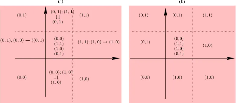
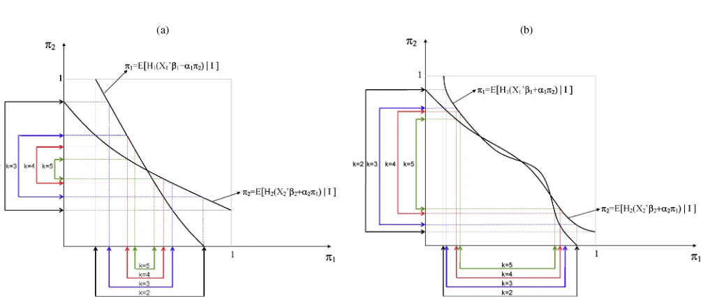
a singleton. Figure 2 shows the mapping between the predic-tions of the game and the observed data under Nash and level-k
rationality. The observable implication of Nash is different de-pending on whether or not we allow for mixed strategies. In particular, without allowing for mixed strategies, in the middle square of Figure 2(a), the only observable implication is(1,0)
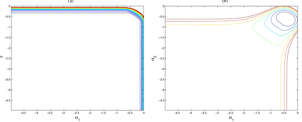
and(0,1); however, it reverts to all outcomes once the mixed strategy equilibrium is considered. To get an idea of the identifi-cation gains when we assume rationality versus equilibrium, we simulated a stylized version of the foregoing game in the case wheretpis standard normal forp=1,2 and the only object of
interest is the vector (α1, α2). We compare the identified set of
the foregoing game underk=1 rationality and NE when we
consider only pure strategies. Figure 3 shows that there is iden-tifying power in assuming Nash equilibrium. In particular, un-der Nash, the identified set is a somehow tight “circle” around the simulated truth, whereas under rationality, the model pro-vides only upper bounds on the alphas. But if we add exoge-nous variations in the profits (X’s), then the identified region under rationality will shrink. In the next section we examine the identifying power of the same game under incomplete in-formation.
4. DISCRETE GAME WITH
INCOMPLETE INFORMATION
Consider now the discrete game presented in Table 1 but un-der the assumptions that player 1 (2) does not observet2 (t1)
or that the signals are private information. We denote player
p∈ {1,2}’s opponent by−p. We letIpdenote the signals used
by playerpto obtain information aboutt−p, wheretp∈Ipcould
be a special case. Player pholds beliefs about his opponent’s type conditional onIp, and those beliefs can be summarized by
a subjective distribution function. Letπ2(I1)denote player 1’s subjectiveprobability of entry for player 2, and defineπ1(I2)
analogously for player 2. Given his beliefs, the expected utility function of player 1 is
U(a1,t1,I1)=
t1+α1π2(I1) ifa1=1
0 otherwise.
Similarly, for player 2, we have
U(a2,t2,I2)=
t2+α1π1(I2) ifa2=1
0 otherwise.
Both players are assumed to be expected-utility maximizers who make choices simultaneously and independently. (This in-cludes NE behavior as a special case.) This yields threshold-crossing decision rules
Y1=1{U(1,t1,I1)≥0}, Y2=1{U(1,t2,I2)≥0}. (2)
Incomplete information makes it impossible for playerpto ran-domize in a way that makes his opponent exactly indifferent be-tween his two actions. In addition, because we focus on the case wheretpis continuously distributed, the eventU(1,tp,Ip)=0
occurs with probability 0. Our assumptions differ from NE
be-(a) (b)
Figure 2. Observable implications of equilibrium (b) versus rationality (a).
(a) (b)
Figure 3. Identification set under Nash and 1-level rationality. Shown the identified regions for(α1, α2)underk=1 rationality (a) and
Nash (b). We set in the underlying model(α1, α2)=(−.5,−.5). The model was simulated assuming Nash with(0,1)selected with probability
one in regions of multiplicity. Note that in (a), the model only places upper bounds on the alphas, whereas in (b)(α1, α2)are constrained to lie
a much smaller set (the inner “circle”).
cause we do not impose the restriction that subjective beliefs are consistent with players’ actual behavior. Again, here we as-sume that bothα1andα2are negative.
4.1 Implications of Level-1 Rationality
We maintain the expected utility maximization assumption and the resulting decision rules (2). In the first round of ratio-nality, we know that for any belief function, or without making any common prior assumptions, the following hold:
t1+α1≥0 ⇒ U(1,t1,I1)=t1+α1π2(I1)≥0
∀π2(I1)∈ [0,1],
(3)
t1≤0 ⇒ U(1,t1,I1)=t1+α1π2(I1)≤0
∀π2(I1)∈ [0,1].
Well-defined beliefs satisfy π2(·)∈ [0,1]. This implies that
if player 1 is an expected-utility maximizer and holds well-defined beliefs, then he must satisfy
t1+α1≥0 ⇒ a1=1
and
t1≤0 ⇒ a1=0.
Now, let 0≤t1≤ −α1. For a player that is rational of order
1, there exists well defined beliefs that rationalizes either 1 or 0. Thus when 0≤t1≤ −α1, both a1=1 and a1=0 are
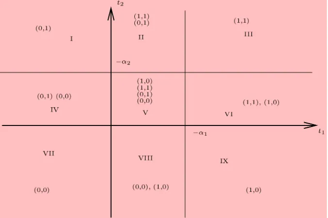
ra-tionalizable. So, the implication of the game are summarized in Figure 4. Note here that the (t1,t2) space is divided into
nine regions: four regions where the outcome is unique, four re-gions with two potentially observable outcomes, and the middle square where any outcome is potentially observed. To make in-ference based on this model, we need to map these regions into predicted choice probabilities. To obtain the sharp set of para-meters that is identified by the model, we can supplement this
model with consistent “selection rules” that specify, in regions of multiplicity, the probability of observing the various out-comes, which would be a function of both(t1,I1)and(t2,I2).
The probabilities can be given a “structural” interpretation in which they would be interpreted as proper selection mecha-nisms. Given the level-1 behavioral assumptions, the only valid selection mechanisms are those that can be produced (rational-ized) by the choice rules (2) for some well-defined beliefs. Ex-pected utility maximization explains [through (2)] how players’ choices are produced in an incomplete information environ-ment given beliefs. Finally, let the joint distribution of(t1,t2)
be noted byF(·).
Result 1. For the game with incomplete information, let the players be rational with order 1 (level-1 rational) and write
Wp≡tp∪Ip. Then the choice probabilities predicted by the
model are
P(1,1)=
III dF+
II
SII(1,1)(W1,W2)dF
+
VI
SVI(1,1)(W1,W2)dF+
V
SV(1,1)(W1,W2)dF,
P(0,0)=
VII dF+
VIII
SVIII(0,0)(W1,W2)dF
(4)
+
IV
S(IV0,0)(W1,W2)dF+
V
SV(0,0)(W1,W2)dF,
P(0,1)=
I dF+
II
SII(0,1)(W1,W2)dF
+
IV
S(VI0,1)(W1,W2)dF+
V
SV(0,1)(W1,W2)dF,
whereSij≥0 are such that for example,SII(1,0)+SII(1,1)=1, and so on, and I, II, III, IV, V, VI, and VIII are regions for(t1,t2)
shown in Figure 4.
Figure 4. Observable implications of level-1 rationality.
The functionsSare unknown and represent “selection” func-tions that represent the probabilities of selecting a particular outcome in a region of multiplicity. Suppose, for simplicity, that
Ip=tp, so that players condition their beliefs only on the
real-ization of their own type. The (sharp) identified setI, is the
set of parameters where there exists proper selection functions
S such that the predicted choice probabilities in (4) are equal to the ones obtained from data. The restrictions in (4) can be exploited by, for example, discretizing the joint distribution of
(t1,t2), such as discussed for the complete-information case,
to construct the identified set. The latter,I, is the set of
pa-rameters for which the equalities in (4) are satisfied for well-defined selection functions. Implications of the foregoing set of equalities is a set of momentinequalitiesconstructed by ex-ploiting the fact that theSfunctions are probabilities and thus are positive. So, for example, an implication of Result 1 is that
IIIdF≤P(1,1)≤
IIIdF+
II∪III∪V∪VIdF, where the bounds
of this inequalities do not involve the unknown functionsS. Next we analyze the behavior of players who assume that their opponents are (at least) level-krational fork≥1. Level-2 rational players are those whose second-order beliefs for their opponent are compatible with the bounds implied by (3). As we show, by eliminating beliefs that violate (3), we are able to reduce the set of level-2 rational beliefs from the entire[0,1] in-terval to a segment of it. Further rounds of iterated thinking will refine these bounds even more. Unlike in the Bayesian Nash equilibrium (BNE) case, we do not impose the requirement that beliefs are correct; we will rule only out those that are not com-patible with the assumption that opponents are level-krational.
4.2 Implications of Level-k Rationality
Level-1 rationality is characterized simply by expected utility maximization and any arbitrary system of well-defined beliefs. We now generalize the results of the previous section by char-acterizing bounds for beliefs that are compatible with assuming
that opponents are level-krational. This means that, for exam-ple, level-2 rational players are all of those whose beliefs are consistent with the bounds implied by (3). As we show later, by eliminating beliefs that violate (3), we will be able to reduce the set of level-2 rational beliefs from the entire[0,1]interval to a segment of it. Level-3 rational players are those whose beliefs are compatible with the bounds for level-2 rational beliefs. This iterative construction can then be used to characterize bounds for level-krational beliefs. Each “round of rationality” refines these bounds by deleting all beliefs that assign positive proba-bility to opponents’ dominated strategies. As a reminder, the re-alization oftpis privately observed by playerp, who conditions
his beliefs about the expected action of his opponent on the re-alization of signals Ip, with tp∈Ip being a special case. The
true distribution of(t1∪t2∪I1∪I2)is common knowledge
to both players. This is the common prior assumption. Even though it plays no role in the analysis of level-1 rational behav-ior, the common prior assumption is important for higher levels of rationality. We consider strategies (decision rules) for player
pthat are threshold functions oftp,
Yp=1{tp≥μp} forp=1,2. (5)
It follows from the normal-form payoffs in Table 1 that this family of decision rules includes those of all expected utility-maximizing players in this simple binary choice game with in-complete information. Level-1 rational players and those who play a BNE are two special cases. In the construction of his ex-pected utility, playerpformssubjectivebeliefs aboutμ−pthat
can be summarized by a probability distribution forμ−pgiven
Ip. These beliefs are derived as part of a solution concept. They
may include BNE beliefs as a special case (in which case all players know those equilibrium beliefs to be correct). Here let
G1(μ2|I1)denote player 1’s subjective distribution function for
μ2givenI1, and define G2(μ1|I2)analogously for player 2.
A strategy by playerpisrationalizableif it is the best response (in the expected-utility sense) given some beliefsGp(μ−p|Ip)
that assign zero probability mass to strictly dominated strategies by player−p. A rationalizable strategy by playerpis described by
where the support S(Gp) excludes values of μ that result in
dominated strategies within the class (5). Throughout, we fo-cus on the case whereμ−pis continuously distributed
condi-tional on Ip, and ignore the distinction between strictly and
weakly dominated strategies. Note that the subset of ratio-nalizable strategies within the class (5) is of the form μp=
−αp
S(Gp)E[1{t−p≥μ}|Ip, μ]dGp(μ|Ip). In this setting, ra-tionalizability requires expected utility maximization for a given set of beliefs but does not require those beliefs to be cor-rect. It only imposes the condition thatS(Gp)exclude values of
μ−p that are dominated. We eliminate such values by iterated
deletion of dominated strategies.
Now we describe the iterative procedure that restrictsS(Gp)
by iterated dominance. As before, we maintain that the signs of the strategic interaction parameters(α1, α2)are known.
Specif-ically, suppose thatαp≤0. Then, repeating arguments from the
previous section onk=1–rationalizable outcomes, looking at
(6), we see that we must have eventwise comparisons
1{tp+αp≥0} ≤1{Yp=1} and
(7)
1{tp<0} ≤1{Yp=0}.
Decision rules that do not satisfy these conditions are strictly dominated for all possible beliefs. Therefore, the subset of strategies within the class (5) that are not strictly dominated must satisfy Pr(tp+αp≥0)≤Pr(tp≥μp)≤Pr(tp≥0) or,
equivalently,μp∈ [0,−αp]. All other values ofμpcorrespond
to dominated strategies. In this setup, we refer that to the subset of strategies that satisfyμp∈ [0,−αp]aslevel-1 rationalizable strategies. Note that, as before, these μ’s do not involve the common prior distributions.
Level-2 rational players are those whose beliefs are consis-tent with assuming that their opponents are level-1 rational. Without any further assumptions, level-2 rational players are those whose beliefs about others satisfy (7). Consequently, a level-2 rational player must have beliefs that assign zero proba-bility mass to valuesμ−p∈ [/ 0,−αp]. As before, we impose no
further requirements (such as having unbiased beliefs). A strat-egy is level-2 rationalizable if it can be justified by level-2 ra-tionalizable beliefs, that is,
level-1–dominated strategies. Moreover, the expectation within the integral is taken with respect to the common prior condi-tional onIp, which includes playerp’s type. Thus, exploiting this monotonicity, it is easy to see that for an outside observer, the subset of level-2 rationalizable strategies must satisfy
μ1∈
Level-krational players are those whose beliefs are consistent with assuming that their opponents are level-(k−1)rational. Note that this definition is a statement about a player’s
higher-order beliefs up to higher-order k−1; specifically, any player who
believes that his opponent undertakes (at least)k−1 rounds of iterated deletion of dominated strategies in the construction of his expected utility will be a level-krational player. By induc-tion, it is easy to prove the following claim.
Claim 1. Ifαp≤0, then a strategy of the typeYp=1{tp≥
The bounds described in (8) contain any set of beliefs that can be rationalized afterk−1 rounds of iterated deletion of dominated strategies. We present identification results based on this entire range with no additional restrictions on how level-k
players actually choose their beliefs from within this space of rationalizable beliefs.
Remark 1. Any level-krational player also is level-k′ ratio-nal for any 1≤k′≤k−1. Also, forp∈ {1,2}, with probability 1, we have that[μLp,k, μUp,k] ⊆ [μLp,k−1, μUp,k−1]for any k>1, with strict inclusion ifαp=0 andt−phas unbounded support
conditional onIp. This monotonic feature of bounds (ask in-creases) is a consequence of the payoff parameterization in the game. Note also that these bounds are a function ofIp, the
in-formation on which playerpconditions his beliefs.
The two statements in Remark 1 follow because conditional onIp, the supportS(Gp)of ak-level rational player is contained
in that of ak−1–level rational player. In fact, if there is a unique BNE (conditional onIp), thenS(Gp)will collapse to the
single-ton given by BNE beliefs ask→ ∞. Whenever warranted, we
clarify whether ak-level rational player is “at mostk-level ratio-nal” or “at leastk-level rational.” For inference based on level-2 rationality, we can use inequalities similar to (4) to map the ob-served choice probabilities to the predicted ones; in particular, we can use the thresholds from Claim 1 to construct a map be-tween the model and the observable outcomes using (5). This is illustrated in Figure 5 for the case whereIp=tp(i.e.,
play-ers condition their beliefs exclusively on the realization of their own type). TherePt1(·)denotes the conditional distribution of
t2|t1, withPt2(·)defined analogously. We see that, moving from
level 1 to level 2, the middle square shrinks. As we show later, higher rationality levels (properly speaking, further rounds of deletion of dominated strategies) will shrink it further. The set of choice probabilities predicted by the model with level-k ra-tional players can be characterized by generalizing Result 1.
Figure 5. Observable implications of level-2 rationality.
Result 2. Let
πpL(1;Ip)=0 and πpU(1;Ip)=1 forp=1,2, and let fork>1,
π1L(k;I1)=E1{t2+α2π2U(k−1;I2)≥0}|I1
,
π1U(k;I1)=E1{t2+α2π2L(k−1;I2)≥0}|I1
,
π2L(k;I2)=E1{t1+α1π1U(k−1;I1)≥0}|I2
,
π2U(k;I2)=E1{t1+α1π1L(k−1;I1)≥0}|I2
.
Using the notation in Section 2, the space of strategies for level-krational players is
Rp(k)=Yp=1{tp+αpπ−p(Ip)≥0}:
π−p∈ [π−Lp(k; ·), π−Up(k; ·)]
forp=1,2.
In the next section we parameterize the typestp to allow for
observable heterogeneity and provide sufficient point identifi-cation conditions based exclusively on the restrictions implied by level-krationality.
4.3 Identification With Level-k Rationality in a Parametric Model
From here on, we expresstp=Xp′βp−εp, whereXp is
ob-servable to the econometrician,εp is not, andβp must be
es-timated (along withαp, the strategic interaction parameter for
playerp). Playerpobserves the realization of his ownXpand
εp, where the latter isonlyprivately observed. We also allow
the possibility that some elements inXpare private information
to playerpand, as before, denote the vector of signals used by playerpto condition his beliefs byIp. Throughout, we assume
(ε1, ε2)to be continuously distributed, with scale normalized to
1 and unbounded support. The results that follow only require that for each playerp, the support ofεpbe larger than that of
Xp′βpfor all possible realizations ofI−p. For simplicity, we
as-sume thatε1is independent ofε2 and denote their cumulative
distribution function (cdf) asHp(·)forp=1,2. Conceptually,
we can extend the result that follow and obtain constructive identification results for the case where ε1 and ε2 are
corre-lated, but we do not deal with that case here. For simplicity, we limit ourselves to the case where beliefs are conditioned on ob-servables to the researcher; that is,Ipis observable. We define
the identified set of parameters and then provide an objective function that can be used to construct the identified set. This function depends on the level kof rationality that the econo-metrician assumes ex ante. We discuss the identification ofk, then we provide a set of sufficient conditions to guarantee point identification under some assumptions. These point identifica-tion results provide insight into the kind of “variaidentifica-tion” needed to shrink the identified set to a point. Our results can be ex-tended to cases where beliefs are conditioned on unobservables to the researcher, as long as the joint distribution of all un-observables in the model is assumed known, possibly up to a finite-dimensional parameter.
As in the previous section, we make a common prior assump-tion. This assumption is only needed to compute bounds on be-liefs for levels of rationality k that are strictly larger than 1.
Specifically, we assume that H1 andH2 are common
knowl-edge among the players, and also assume that the econometri-cian knows these common prior distributions. We assume that players use the true distributions as their priors for payoff co-variatesXp and signalsIp, both of which are observed by the
econometrician. Implicitly, we also assume that the true values
of βp andαp are common knowledge to both players. Given
this setup, we can construct bounds on beliefs iteratively. For any parameter value and any “rationality level,” these bounds are identified, and they constitute the foundation for our identi-fication results.
Iterated Dominance and Bounds for Beliefs. For ease of ex-position, we assume that both players condition on the same
vector of signals, which we denote byI. This would include the
case where the only source of private information for playerpis
εpandI=X1∪X2. We will return to the more general case and
allow forI1=I2later. As in Section 4.2, we derive bounds for
the range of rationalizable beliefs iteratively by deleting those that assign positive probability to opponents’ dominated strate-gies. For each playerp, let
π−Lp(θ|k=1,I)=0, and πU
−p(θ|k=1,I)=1,
and fork≥2, let
π1L(θ|k,I)=EH1
X1′β1+α1π2U(θ|k−1,I)
|I;
(9)
π1U(θ|k,I)=EH1
X1′β1+α1π2L(θ|k−1,I)
|I;
π2L(θ|k,I)=EH2
X2′β2+α2π1U(θ|k−1,I)
|I;
π2U(θ|k,I)=EH2
X2′β2+α2π1L(θ|k−1,I)
|I,
where π−Lp(θ|k,I) and π−Up(θ|k,I) are the lower and up-per bounds for level-k rationalizable beliefs by player p for Pr(Y−p|I). Given our foregoing assumptions, these bounds are
identified for anyθandk. In the case where we want to allow for correlation inε1andε2, the belief function for playerpwill
depend onεp, which would be part of a player-specific
infor-mation set, andHpwould be the conditional cdf ofεp|ε−p. By
induction, it is easy to show that
[π−Lp(θ|k;I), πU
−p(θ|k;I)]
⊆ [π−Lp(θ|k−1;I), π−Up(θ|k−1;I)]
with probability 1 inS(I). (10)
This monotonic feature holds even if players condition on dif-ferent information sets. Moreover, the inclusion in (10) is strict if the strategic interaction coefficients are nonzero and ifεphas
unbounded support conditional onX′pβpandI. Figure 6 depicts
this case for a fixed realizationI, a given parameter vectorθ,
andk∈ {2,3,4,5}.
Identified Set forθBased on Level-k Rationality. LetWp= Xp∪I. It follows from the discussion in Section 4.2 (see
Re-sult 2) that the identified set forθ under the assumption that players are level-krational is given by
I(k)=
θ∈:∃π1(·), π2(·)∈ [π1L(θ|k; ·), π1U(θ|k; ·)]
× [π2L(θ|k; ·), π2U(θ|k; ·)]
such thatE[Yp|Wp] =Hp(Xp′βp+αpπ−p(I))
with probability 1 forp=1,2. (11)
We exploit the fact that under our assumptions, the bounds for level-k rational beliefs are identified to characterize a set
(k)that includesI(k). Our characterization constructive and
based on conditional moment inequalities. To proceed, note that playerpis level-krational if and only if
1{Xp′βp+αpπ−Up(θ|k;I)≥εp}
≤1{Yp=1}
≤1{Xp′βp+αpπ−Lp(θ|k;I)≥εp} with probability 1.
Recall that we are studying the case whereαp≤0 forp=1,2.
These inequalities must hold with probability 1 for all realiza-tions of(Xp, εp,I). It follows that level-krational players must
satisfy
Hp
Xp′βp+αpπ−Up(θ|k;I)
≤E[Yp|Wp]
≤Hp
Xp′βp+αpπ−Lp(θ|k;I)
with probability 1,
whereWp=Xp∪I. Define the set
(k)=θ∈:Hp
Xp′βp+αpπ−Up(θ|k;I)
≤E[Yp|Wp]
≤Hp(X′pβp+αpπ−Lp(θ|k;I))
with probability 1,p=1,2. (12)
(a) (b)
Figure 6. Rationalizable beliefs fork=2,3,4, and 5. (a) Belief iterations with a unique BNE. (b) Belief iterations with a multiple BNE. Bounds for level-krationalizable beliefs whenI1=I2≡I (players condition on the same set of signals). The vertical axis shows level-k
rationalizable bounds for player 1’s beliefs about Pr(Y2=1|I). The horizontal axis shows the equivalent objects for player 2. The graphs
correspond to a particular realizationIand a given parameter valueθ.
Clearly, if players are level-krational, then we have I(k)⊆
(k). If Xp ∈ I for both players, then it is easy to show
that I(k)=(k). This follows because the set [π1L(θ|k; ·),
π1U(θ|k; ·)] × [π2L(θ|k; ·), π2U(θ|k; ·)]is connected and the dis-tributionsH1andH2are continuous. The characterization(k)
is constructive and is the one that we use even though it might be a strict superset of the sharp set 2(k). This is because
dealing with the set (k) is simple and computationally
at-tractive. To allow for the case whereWp has continuous
sup-port, we reexpress(k)as the set of minimizers of an objective function (see Dominguez and Lobato 2004). For two vectors
a,b∈Rdim(Wp), let This is the definition of identified set forθ that we use under the assumption that all players in the game are level-krational. More precisely, returning to Remark 1,(k)is the identified set if we assume that all players in the population are at least level-k rational. By construction, (k+1)⊆(k) for all k. Methods meant for set inference can be adapted to construct a
sample estimator of(k)based on a random sample of games
where all players are level-krational for a givenk. Note also that, compared with the Bayesian Nash solution, here we do not need to solve a fixed-point map to obtain the equilibrium; rather, rationalizability requires restrictions on player beliefs, which can be implemented iteratively. We formally show that
(k)contains the set of BNE for anyk>0. Having(k)= ∅
would reject the hypothesis that all players are at least level-k
rational.
Remark 2. Note that when k=1, we do not need to spec-ify the common prior assumption, because here beliefs play no role. Thus results will be robust to this assumption. However, depending on the magnitude of theαp’s, the bounds on choice
probabilities predicted by such a model (wherek=1) can be
wide.
Under certain conditions, the identified set in (14) would con-sist only ofθ0, the true parameter value. An example of this is a
case in which there exist realizations of the vector of signalsI
where the players are “forced” to take one of their actions with probability 1 regardless of their beliefs. To be concrete, suppose that the linear indexX′pβphas unbounded support for both
play-ers, and suppose that both of them are at least level-2 rational (i.e., they both perform at least one round of deletion of dom-inated strategies). Then, if the vector of signalsI is such that
there exist regions ofS(I)such thatS(Xp′βp|I)is concentrated
around arbitrarily large positive or arbitrarily large negative val-ues, the identified set(k=2)defined in (14) would collapse to a singletonθ0, the true parameter value. We refer to this as a
case of “informative signals” and formalize this point identifi-cation result in the next section.
4.4 Sufficient Point Identification Conditions
In this section we study the problem of point identification of the parameter of interests in the foregoing game. In particular, we provide sufficient point identification conditions for level-1 rational play and for levelsk>1. These conditions can provide insight into what is required to shrink the identified set to a point (or a vector). Here we allow for the information sets to
be different; that is, player p conditions on Ip when making
decisions and allow for exclusion restrictions whereI1=I2.
We start with sufficient conditions for level-1 rationalizability.
4.4.1 Identification Results With Level-1 Rationality. Let
θp=(βp, αp)andθ=(θ1, θ2); then we have the following
iden-tification result.
Theorem 1. Suppose thatXphas full rank forp=1,2, and let X≡(X1,X2); assume thatαp<0 forp=1,2, and letdenote
the parameter space. Let there be a random sample of size N
from the foregoing game. Consider the following conditions:
A1.1 For each playerp, there exists a continuously distrib-utedXℓ,p∈Xp with nonzero coefficientβℓ,p and
un-bounded support conditional onX\Xℓ,psuch that for
anyc∈(0,1),b=0, andq∈Rdim(X−ℓ,p), there exists Cb,q,m>0 such that
Pr(εp≤bXℓ,p+q′X−ℓ,p|X) >m
∀Xℓ,p: sign(b)·Xℓ,p>Cb,q,m. (15)
A1.2 For p=1,2, letXd,p denote the regressors that have
bounded support but are not constant. Suppose that
is such that for anyβd,p,βd,p∈withβd,p=βd,pand If all we know is that players are level-1 rational, then the fol-lowing hold:
a. If (A1.1) holds, then the coefficientsβℓ,pare identified.
b. If (A1.2) holds, then the coefficientsβd,pare identified.
c. We say that player p is pessimistic with positive proba-bility if for any >0, there existsX∈S(Xp)such that
Pr(Yp=1|X) <Pr(εp≤Xp′βb0 +αp0|X)+ whenever
Xp∈X. If (A1.1) and (A1.2) hold and playerpis
pes-simistic with positive probability, then the identified set forαpis{αp∈:αp≤αp0}. (Here we refer to the
identi-fied set as the set of values ofαpthat are observationally
equivalent, conditional on observables, to the true value
αp0.)
The results in Theorem 1 imposed no restrictions onIp. In
particular, players can condition their beliefs on unobservables to the econometrician. A special case of condition (A1.1) is whenεpis independent ofX. The condition in (A1.2) says how
rich the support of the bounded shifters must be in relation to
the parameter space. Covariates with unbounded support satisfy this condition immediately given the full-rank assumption. Fi-nally, similar identification results to Proposition 1 hold for the cases whereαp≥0 andα1α2≤0. The proof of Theorem 1 is
given in the Appendix.
4.4.2 Identification With Level-k Rationality. We now move on to the case of rationalizable beliefs of higher order. Our goal is to investigate whether a higher degree of rationality will the task of point-identifying αp. To simplify the
analy-sis, we assume from here on thatεpis independent ofXand of
I≡(I1,I2). This assumption could be replaced with one along
the lines of (A1) in Theorem 1. We make the assumption thatI
is observed by the econometrician; we relax it later. Again, de-note the common prior assumption byHp(·). The beliefs of the
players for any level-krationality can be constructed as done in the previous section. Our point identification–sufficient condi-tions are summarized in Theorem 2.
Theorem 2. Suppose that there exists a subset X∗
1 ⊆S(X1)
whereX1has full-column rank such that for anyX1∈X1∗,ε >
0, andθ2∈, there existℑ∗1ε ⊂S(I1|X1)andℑ∗∗1ε ⊂S(I1|X1)
such that
for allI1∈ ℑ∗
1ε,
max1−E[H2(X2′β2+2)|I1],
E[H2(X′2β2+2)|I1] −E[H2(X2′β2+2+α2)|I1]
< ε,
(17) for allI1∈ ℑ∗∗1
ε,
maxE[H2(X2′β2+2+α2)|I1],
E[H2(X′2β2+2)|I1] −E[H2(X2′β2+2+α2)|I1]
< ε.
A special case in which (17) holds is when there existsX2ℓ∈
(X2∩W1) with nonzero coefficient in such that X2ℓ has
unbounded support conditional on (X2∪W1)\X2ℓ. We can
call (17) an “informative signal” condition. Note that implicit in (17) is an exclusion restriction in the parameter space that precludes β2=0 for any θ2∈. If (17) holds, then for any
θ∈ such thatθ1=θ10, there exists eitherW ∗
1 ⊂S(W1)or
W∗∗
1 ⊂S(W1)such that
H1X′1β1+1+α1π2L(θ|k;I1)
<H1
X1′β10+10+α10π
U
2(θ0|k;I1)
∀W1∈W1∗,k≥2;
(18)
H1
X′1β1+1+α1π2U(θ|k;I1)
>H1
X1′β10+10+α10π
L
2(θ0|k;I1)
∀W1∈W1∗∗,k≥2.
Therefore, for anyk≥2, the level-krationalizable bounds for player 1’s conditional choice probability ofY1=1|W1that
cor-respond to θ will be disjoint with those of θ0 with positive
probability. Consequently, if (17) holds and the population of player 1’s are at least level-2 rational,θ10 is identified. By
sym-metry,θ20 will be point-identified if the foregoing conditions
hold, with the subscripts “1” and “2” interchanged.
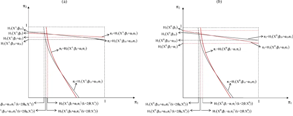
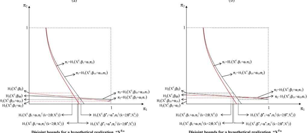
For the case in whichI1=I2=Xand the only source of pri-vate information in payoffs isεp, Figures 7 and 8 illustrate four
graphical examples of how the “informative signals” condition (17) in Theorem 2 yields disjoint level-2 bounds.
The ability to shift the upper and lower bounds for level-2 rationalizable beliefs arbitrarily close to 1 or 0 is essential for the point-identification result in Theorem 2. For simplicity, the intercept1is subsumed inX1′β1in the labels of these figures.
4.5 On Identification of Players’ Rationality Level
Without further structure, our setup is not capable of identi-fying each individual player’s rationality level (measured byk). Furthermore, without strong assumptions about the support of
εprelative to that ofXp′βp, it is not possible to reject a value of
(a) (b)
Figure 7. Graphical examples of informative signals, I.
(a) (b)
Figure 8. Graphical examples of informative signals, II.
kon the basis of observed choices. But our setup is capable of producing identification results for the valuek0such that
play-ers in the population are at most level-k0rational. This refers
to the value such that the level-k0 bounds hold with
probabil-ity 1, but the level-(k0+1)bounds are violated with positive
probability in the population. In other words, our setup has the potential to identify the rationality levelk0such that a portion
of players in the population have beliefs that violate the
level-(k0+1) rationalizable bounds. Whether or not we can
iden-tifyk0 depends on how much we can identify about θ. If all
players are at least level-2 rational and the conditions for point identification ofθdescribed in Theorem 2 hold, thenk0would
be point-identified becauseQ(θ0|k)=0 if and only if k≤k0,
whereQ(θ|k)is as defined in (14). To see why this is not true whenθis set-identified, refer to parts (a) and (b) following (19). Otherwise, if the conditions for Theorem 2 do not hold, then
suppose that we maintain the assumptionk0≥1 (the only
in-teresting case). We can start withk=1 and construct(1), as defined in (14). Next, for anyk≥2, define
Q(k)= min
θ∈(1)Q(θ|k), (19)
whereQ(θ|k)is as defined in (14). Then the following hold: a. Q(k)=0 for allk≤k0; however,Q(k)=0 does not imply,
k≤k0.
b. Q(k) >0 implies thatk>k0.
Suppose that different observations in the data set correspond to a game with a different level of rationality; then ifQ(k) >0 and
Q(k−1)=0, we would reject the hypothesis (strictly speaking, this would be a joint test of the rationality hypothesis and all other maintained assumptions) that all of the population is at least level-k rational. If we assumed ex ante thatk0≥k>1,
then we could simply replace(1)with(k)in the definition ofQ(k)in (19). Alternatively, in settings where at least a subset of the structural parameterθ is known (e.g., experiments), we could evaluate whether players are at least level-k0rational by
testing whether or notθ0∈(k0)(the identified set for level-k0
rationality). Otherwise, a test that would fail to reject (k0+
1)= ∅would indicate that players are at most level-k0rational.
4.6 Bayesian Nash Equilibria and Rationalizable Beliefs
As before, let Ip be the signal that player p uses to con-dition his beliefs about his opponent’s expected choice, and
let I ≡(I1,I2). The set of BNE is defined as any pair
(π1∗(I2), π2∗(I1))≡π∗(I)that satisfies
π1∗(I2)=EH1(X1′β1+α1π2∗(I1))|I2
,
(20)
π2∗(I1)=EH2(X2′β2+α2π1∗(I2))|I1
.
By construction, the set of rationalizable beliefs forImust
in-clude the BNE set for any rational levelk. The following result formalizes this claim.
Proposition 1. Let
R(I;k)= [π1L(θ|k;I2), π1U(θ|k;I2)]
× [π2L(θ|k;I1), πU
2(θ|k;I1)]
denote the set of level-krationalizable beliefs. Then, with prob-ability 1, the BNE set described in (20) is contained inR(I;k)
forany k≥1.
We present the proof for the case whereαp≤0 forp=1,2,
on which we have focused. The proof can be adapted to all other cases. We proceed by induction by first proving the following claim.
Claim 2. Letπ∗(I)≡(π∗
1(I2), π2∗(I1))be any BNE. Then,
for anyk≥1, with probability 1, we have thatπ∗(I)∈R(I;k)
implies thatπ∗(I)∈R(I;k+1)with probability 1.
Proof. If αp =0 for p = 1 or p =2, then the result
follows trivially. Suppose that α1=0; then π1L(θ|k;I2)=
π1U(θ|k;I2)=π1∗(I2)=E[H1(X1′β1)|I2] and π2L(θ|k;I1)=
π2U(θ|k;I1)=π2∗(I1)=E[H2(X2′β2+α2π1∗(I2))|I1] for all