T H E J O U R N A L O F H U M A N R E S O U R C E S • 47 • 1
Building the Stock of
College-Educated Labor Revisited
David L. Sjoquist
John V. Winters
A B S T R A C T
In a recent paper in theJournal of Human Resources,Dynarski (2008) used data from the 1 percent 2000 Census Public Use Microdata Sample (PUMS) files to demonstrate that merit scholarship programs in Georgia and Arkansas increased the stock of college-educated individuals in those states. This paper replicates the results in Dynarski (2008) but we also find important differences in the results between the 1 percent and 5 per-cent PUMS, especially for women. We also demonstrate that the author’s use of clustered standard errors, given the small number of clusters and only two policy changes, severely understates confidence intervals.
I. Introduction
Beginning in the early 1990s, several states introduced merit-based financial aid programs for students pursuing higher education within their state of residence. These programs usually have three related goals. First, they aim to in-crease access to higher education and incline some high-achieving high school stu-dents to go to college who might not have been able to afford to do so otherwise. Second, merit programs aim to encourage more students to go to college in-state. Third, these merit programs aspire to increase the completion rate. Several studies have examined the various effects of these merit aid programs, with much of the research focusing on Georgia’s HOPE Scholarship program. Dynarski (2000; 2004) finds that the HOPE Scholarship increased the probability of enrollment for young
David L. Sjoquist is professor of economics and Dan E. Sweat Distinguished Chair in Educational and Community Policy in the Andrew Young School of Policy Studies at Georgia State University. John V. Winters is an assistant professor of economics at the University of Cincinnati. The authors wish to thank Barry Hirsch and participants in the Public Economics Brownbag Series at Georgia State University for helpful comments; the usual caveat applies. The data used in this article can be obtained beginning August 2012 through July 2015 from John Winters at Department of Economics, University of Cincin-nati, P.O. Box 210371, CincinCincin-nati, OH 45221–0371, john.winters@uc.edu.
[Submitted April 2010; accepted March 2011]
people in Georgia.1In a frequently cited paper in theJHR, Dynarski (2008) examines
microdata from the 2000 Census and concludes that merit aid programs in Georgia and Arkansas have increased the share of young people who have obtained a college degree (either an associate’s or bachelor’s) by three percentage points.
This paper replicates Dynarski (2008) and explores the sensitivity of her results to using a different sample and different estimation procedures. Several interesting results emerge. First, coefficient estimates differ between the 2000 Census 1 percent Public Use Microdata Sample (PUMS) and the 5 percent PUMS. Using the 1 percent PUMS with Dynarski’s estimation procedures (which are explained in detail in her article), we are able to replicate her results exactly. However, when Dynarski’s es-timation procedure is applied to the 5 percent PUMS, the coefficient estimates are considerably smaller. The estimated effect of the state merit aid programs on degree completion is 0.0298 using the 1 percent PUMS, but falls to 0.0091 when the 5 percent PUMS is used. Further analysis reveals that the differences across the sam-ples are mostly concentrated among women. Given that the 1 percent and 5 percent PUMS are drawn from the same underlying population, differences across the two samples are largely unexpected.
Our second main result is that the statistical significance levels in Dynarski (2008) are greatly overstated because of her use of clustered standard errors with only two policy changes and with a small number of clusters. Clustered standard errors are often an improvement over Ordinary Least Squares (OLS) standard errors in many applications because conventional OLS standard errors do not account for intraclus-ter correlation and can be downwardly biased. With clusintraclus-tered standard errors there is also the issue of at what level the data should be clustered, for example, at the state level or the state-age level. If there is correlation within states across ages, then clustering at the state level might be preferable for some applications. However, clustered standard errors can also be substantially downwardly biased when the number of clusters is small (MacKinnon and White 1985; Bertrand, Duflo, and Mullainathan 2004; Donald and Lang 2007) or the number of treated groups (policy changes) is small (Bell and McAffrey 2002; Abadie, Diamond, and Hainmueller 2010; Conley and Taber 2011). This small sample bias for clustered standard errors is likely to be especially severe in difference-in-differences models with only a few policy changes (Conley and Taber 2011). To obtain valid inferences, we follow two separate approaches for examining significance levels. First, we address the issue of the small number of policy changes using the approach suggested by Conley and Taber (2011). We then address the small number of clusters using the approach suggested by Cameron, Gelbach, and Miller (2008). Using each of these methods, we find a statistically insignificant effect of merit programs on degree completion for both the 1 percent and 5 percent PUMS. In other words, while the coefficient
272 The Journal of Human Resources
estimates are positive, we cannot be reasonably confident that the true effects are statistically different from zero.
The paper proceeds as follows. In the next section we briefly summarize Dynarski (2008). In Section III we discuss our results using her procedures for the 1 percent and 5 percent PUMS. In Sections IV and V we employ two alternative procedures for inferences suggested by Conley and Taber (2011) and by Cameron, Gelbach, and Miller (2008), respectively. Section VI further investigates differences between the census samples, and a final section concludes.
II. Summary of Dynarski (2008)
Arkansas and Georgia introduced large, broad-based merit-based stu-dent aid programs in 1991 and 1993, respectively.2Dynarski examines the effects
of these two broad-based merit aid programs on degree completion using a treatment-comparison research design. She treats the adoption of merit aid programs in Ar-kansas and in Georgia as natural experiments. Students who finished high school in Arkansas and Georgia after the programs were adopted are considered the treatment group, while the comparison group consists of students in states that did not adopt merit programs during the period under study and students in Arkansas and Georgia who finished high school before the merit programs were implemented.
As a practical matter, the Census microdata do not report when or in what state a student completes high school. Since she does not know who received student aid, Dynarski uses a variable, denotedmerit, which measures whether the student would have been exposed to a merit-based aid program while in high school. This variable is determined by place of birth, not place of residence at the time of the Census, because a change in the percentage of the population with a college degree in a state could be due to migration of college graduates. Given that most students graduate high school at age 18, she assumes that high school graduation occurs at age 18, and thus defines the treatment group as persons who were either (1) born in Arkansas and age 27 or younger at the time of the Census or (2) born in Georgia and age 25 or younger at the time of the Census. Dynarski notes that this assignment of the treatment status will cause measurement error and result in downwardly biased es-timates of the effects of merit programs on degree completion. The sample is then restricted to persons between the ages of 22 and 34 at the time of the 2000 Census, who were born in the United States and have nonimputed information for age, state of birth and education. The sample also excludes persons born in Mississippi because Mississippi adopted a merit program in 1996 and is therefore not a legitimate control group.
Dynarski’s baseline empirical model is represented as follows:
y¯ ⳱merit Ⳮ␦Ⳮ␦ Ⳮε ,
(1) ab ab a b ab
where y¯ab is the share of persons of age a born in stateb who have completed a college degree (either an associate’s or bachelor’s),meritab is an indicator variable
equal to one for the treatment group and zero otherwise,␦aand␦bare age and state of birth fixed effects, andε is an idiosyncratic error term. If the model is correctly
ab
specified, then measures the effect of merit programs on degree completion. Dy-narski (2008) estimates Equation 1 using Weighted Least Squares where age-state observations are weighted by the number of persons in the age by state of birth cells and standard errors are clustered by state of birth.3To estimate Equation 1, she uses
the 1 percent PUMS file from the 2000 Census of Population.
In her baseline results Dynarski obtains a coefficient on the treatment dummy of 0.0298 with a standard error of 0.0040, implying that the merit-based aid programs had a positive and statistically significant effect on college degree attainment. She runs several robustness checks, including the use of different sets of control vari-ables, and obtains similar results: a coefficient of about 0.03 and a standard error of about 0.004.
III. Replication of Dynarski’s Results
We first replicate Dynarski (2008) using the 1 percent PUMS, and then replicate her procedure using the 5 percent PUMS and five 1 percent subsamples created from the 5 percent PUMS. These data were extracted from the IPUMS (Ruggles et al. 2008). For the dependent variable, Dynarski focuses on the comple-tion of an associate’s degree or higher, and we do so as well. We also explore using bachelor’s degrees or higher as the dependent variable (not shown) and find quali-tatively similar results. Table 1 presents our replication results for the 1 percent PUMS, the 5 percent PUMS, and five 1 percent subsamples created from the 5 percent PUMS. The first column presents results for the total population, while the second and third columns present separate results for females and males. The results for the 1 percent PUMS are presented first. We obtain a coefficient estimate for the total population of 0.0298, which is exactly the same as in Dynarski’s baseline specification in Column 1 of her Table 3. Estimating standard errors by clustering by state of birth yields a standard error of 0.0040, the same as in Dynarski (2008). This results in a 95 percent confidence interval between 0.0223 and 0.0374 and implies a statistically significant effect of merit aid programs on degree completion. When we replicate Dynarski’s procedure, but use the 5 percent PUMS, the co-efficient estimate for the total population decreases considerably to 0.0091. Cluster-ing by state of birth produces a standard error of 0.0034, which gives a 95 percent confidence interval between 0.0026 and 0.0157; the effect of merit programs on degree completion is still statistically different from zero using clustered standard errors. However, the difference in the results between the two samples is a bit puzzling. In fact, the difference in the coefficients is sufficiently large and the clus-tered standard errors are sufficiently small that we would reject the null hypothesis that the two samples produce the same merit program coefficient with ap-value less than 0.01. Similarly, the 95 percent confidence intervals for the two estimates do not overlap when based on clustered standard errors.
274 The Journal of Human Resources
Table 1
OLS Estimates of the Effect of Merit Aid Programs on College Degree Attainment, Adults Aged 22–34, 2000 PUMS
Coefficient Estimate on the Merit Aid Program Dummy Variable (Standard Cluster by State 95 Percent Confidence Interval)
{Conley and Taber 95 Percent Confidence Interval} [Cameron, Gelbach, and Miller Wild Cluster P-Value]
Sample Total Population Females Only Males Only
1 percent PUMS 0.0298 0.0377 0.0201
(Replication of Dynarski 2008)
(0.0223, 0.0374) (0.0270, 0.0485) (0.0053, 0.0349) {ⳮ0.0110, 0.0798} {ⳮ0.0317, 0.0925} {ⳮ0.0206, 0.0865}
[p⳱0.168] [p⳱0.194] [p⳱0.222]
5 percent PUMS 0.0091 0.0022 0.0157
(0.0026, 0.0157) (ⳮ0.0057, 0.0102) (0.0096, 0.0218) {ⳮ0.0183, 0.0489} {ⳮ0.0205, 0.0435} {ⳮ0.0186, 0.0628}
(0.0054, 0.0390) (ⳮ0.0083, 0.0417) (0.0010, 0.0510) {ⳮ0.0171, 0.0946} {ⳮ0.0194, 0.0942} {ⳮ0.0227, 0.1100}
[p⳱0.204] [p⳱0.594] [p⳱0.208] 5 percent subsamples
ending 5 & 0
0.0215 0.0082 0.0342
(0.0050, 0.0380) (ⳮ0.0170, 0.0333) (0.0089, 0.0595) {ⳮ0.0085, 0.0643} {ⳮ0.0406, 0.0425} {ⳮ0.0074, 0.0949}
[p⳱0.212] [p⳱0.208] [p⳱0.214]
Given that the Census samples are drawn from the same underlying population, this difference in coefficients is unexpected. However, there is likely a problem with using clustered standard errors to make inferences in this setting. Inferences using clustered standard errors are based on the assumption of a large number of treatment groups. However, clustered standard errors are considerably downwardly biased in difference-in-differences models that are based on a small number of policy changes (Conley and Taber 2011). Thus, it is likely that the clustered standard errors are underestimated and lead to invalid inferences. Furthermore, larger standard errors could help explain the differences in coefficient estimates for the different samples. Larger standard errors could mean that the differences across the samples are not statistically significant, and we would be less surprised to find moderately different coefficient estimates from different samples.
As further evidence that results might differ across samples, we explored dividing the 5 percent PUMS into five 1 percent subsamples using the PUMS subsample variable. Both the 1 percent and the 5 percent PUMS divide the population into 100 random subsamples numbered from 0 to 99 (U.S. Bureau of the Census 2003). The 5 percent PUMS can, therefore, be divided into five 1 percent subsamples using this variable. We follow Census recommendations and construct five 1 percent subsam-ples by grouping subsamsubsam-ples ending in 1 and 6, 2 and 7, 3 and 8, 4 and 9, and 5 and 0 (p. 95). We then estimate the effect of merit-aid programs on degree comple-tion using the same procedure as Dynarski (2008) for each sample. These results are also presented in Table 1. For the first three constructed 1 percent subsamples, the estimated coefficients for themeritvariable are very small and not statistically significant using clustered standard errors. For the fourth and fifth constructed 1 percent subsamples, however, the coefficient estimates are 0.0222 and 0.0215, re-spectively, and are significant at the 5 percent level using clustered standard errors. Again, these constructed samples are drawn from the same underlying population and should not give statistically significantly different results. However, because clustered standard errors are likely underestimated, we should not use them for making inferences in this instance; we return to this in the next section.4
Dynarski (2008) also suggests that there are important differences by gender in the effects of merit programs on degree completion. She finds that the effect for women is roughly twice as large as the effect for men. We next estimate separate effects by gender for the various samples that we use. An interesting result emerges in that most of the difference between the 1 percent and 5 percent PUMS is due to females. The merit coefficient for females is 0.0377 in the 1 percent PUMS, but only 0.0022 in the 5 percent PUMS. This is an even bigger difference than for the total population. For males, though, themeritcoefficient estimates are only slightly different across the two samples at 0.0201 and 0.0157 for the 1 percent and 5 percent PUMS, respectively. However, coefficient estimates differ across the five constructed 1 percent subsamples for both females and males. The merit coefficients range from
276 The Journal of Human Resources
ⳮ0.0071 to 0.0167 for females and fromⳮ0.0050 to 0.0342 for males. Importantly though, conventional clustered standard errors should not be used to determine if the differences across the samples are statistically significant. In the next two sections we follow two approaches intended to provide correct inferences about the effects of merit programs on degree completion. These approaches will also help us discern whether the differences across samples are significant.
IV. Inferences Based on the Conley and Taber
Procedure
As an alternative to using clustered standard errors to make infer-ences, we first implement a procedure suggested by Conley and Taber (2011) using code available from Conley’s website. The Conley-Taber procedure is especially useful in applications where there are a large number of control groups but only a small number of policy changes. Their procedure can be used to estimate confidence intervals in difference-in-differences models based on the distribution of residuals across the control groups. Monte Carlo analysis confirms that their approach out-performs conventional clustering methods when the number of treatment groups is small and does no worse in more general settings. They also illustrate their procedure using the effect of merit aid programs on college enrollment along the lines of Dynarski (2000; 2004) and show that inferences based on their method differ from those based on conventional clustered standard errors. We refer the reader to their paper for further details.
We apply the Conley-Taber (CT) procedure to construct 95 percent confidence intervals for the effect of merit programs on degree completion. These confidence intervals for each merit coefficient estimate are also reported in Table 1. In clear contrast to the standard cluster confidence intervals, the CT confidence intervals include zero for all of the samples considered. In other words, the CT procedure suggests that the effect of the merit programs on degree completion is not significant at the 5 percent level. The effects are also not significant at the 10 percent level (not shown). Furthermore, the CT confidence intervals for the 1 percent and 5 per-cent PUMS have considerable overlap, suggesting that the differences between the coefficients are not statistically significant. The same is true for the five 1 percent subsamples from the 5 percent PUMS. These results hold for the total population as well as females and males separately. This supports the earlier hypothesis that the use of typical clustered standard errors causes significance levels to be consid-erably overstated and results in invalid inferences.
V. Inferences Using the Cameron, Gelbach, and Miller
Wild Cluster Bootstrap
methods compute significance levels by creating many pseudo-samples, estimating the model parameters for each pseudo-sample, and then examining the distribution of the parameters across the various pseudo-samples. The wild cluster bootstrap-t
constructs pseudo-samples by holding the regressors constant while resampling with replacement group-specific residuals to form new dependent variables. The proce-dure also uses Rademacher weights ofⳭ1 andⳮ1, each with a probability of 0.5.
This creates pseudo-samples with dependent variables created using randomly drawn residuals half the time and the negative of the randomly drawn residuals the other half of the time. For each pseudo-sample, the dependent variable is then regressed on the explanatory variables. Significance levels are computed based on the number of times the pseudo-sample coefficients differ from the null hypothesis. Cameron, Gelbach, and Miller (2008) show using Monte Carlo simulations that tests based on the wild cluster bootstrap-t procedure have the appropriate size and provide valid inferences. See their paper for further details.
Table 1 also reports p-values using the Cameron, Gelbach, and Miller (CGM) wild cluster bootstrap-tprocedure. For all of the samples considered, the p-values are at least greater than 0.10, suggesting that the effect of the merit programs on degree completion is not statistically significant at the 10 percent level. In other words, we cannot be reasonably confident that merit-aid programs have an effect on completion of at least an associate’s degree. In results not shown, we also used the wild cluster bootstrap-tprocedure to examine whether the differences in coefficients between the 1 percent and 5 percent PUMS are statistically significant. The differ-ences are insignificant at the 10 percent level for the total population and for females and males separately. The CGM wild cluster bootstrap-t procedure thus provides inferences similar to the Conley-Taber procedure, but very different from using clus-tered standard errors.
VI. Sample Means and Differences across Samples
While the differences in themeritcoefficients across samples are not statistically significant using the CT and CGM methods, the differences are still large in magnitude, especially for females, and seem to warrant further exploration of the data. Table 2 presents sample means and standard errors for females ages 22– 34 for several variables by state of birth for the 1 percent and 5 percent samples.5
The upper panel (A) reports means and standard errors constructed without using person weights, while the lower panel (B) does use person weights. There are often important differences between the weighted and unweighted means. While there is not agreement on this, many applied econometricians argue that when possible, researchers should use the person weights. Dynarski (2008) does not use person weights and neither do our results in Table 1. We also reestimated our main results using the person weights to ensure that this is not the cause of the differences in the coefficients (Table 3). The estimates change only slightly and the qualitative
278
The
Journal
of
Human
Resources
Table 2
Means and Standard Errors for Females by State of Birth, 1 percent and 5 percent PUMS
State of Birth: Arkansas Georgia Rest of United States
Mean Standard Error Mean Standard Error Mean Standard Error
A. Unweighted 1 percent PUMS
Associate’s degree or higher 0.2379 0.0096 0.2874 0.0061 0.3555 0.0011 Bachelor’s degree or higher 0.1776 0.0086 0.2166 0.0056 0.2662 0.0010 Nonwhite or Hispanic 0.2318 0.0095 0.3577 0.0065 0.2507 0.0010 Living in birth state 0.6437 0.0108 0.7446 0.0059 0.6686 0.0011
Merit 0.4372 0.0112 0.2921 0.0062 0.0000 0.0000
5 percent PUMS
Associate’s degree or higher 0.2544 0.0044 0.2816 0.0027 0.3567 0.0005 Bachelor’s degree or higher 0.1872 0.0039 0.2179 0.0025 0.2677 0.0005 Nonwhite or Hispanic 0.2409 0.0043 0.3556 0.0029 0.2481** 0.0004 Living in birth state 0.6599 0.0047 0.7476 0.0027 0.6669 0.0005
Merit 0.4571 0.0050 0.2898 0.0028 0.0000 0.0000
Chi-square test statistic 9.04 4.26 8.46
Sjoquist
and
W
inters
279
Associate’s degree or higher 0.2566 0.0115 0.3052 0.0071 0.3696 0.0012 Bachelor’s degree or higher 0.1954 0.0105 0.2337 0.0066 0.2819 0.0012 Nonwhite or Hispanic 0.2576 0.0117 0.3597 0.0074 0.2664 0.0012 Living in birth state 0.6427 0.0125 0.7275 0.0069 0.6579 0.0012
Merit 0.4609 0.0131 0.3004 0.0071 0.0000 0.0000
5 percent PUMS
Associate’s degree or higher 0.2699 0.0052 0.2997 0.0032 0.3706 0.0006 Bachelor’s degree or higher 0.2038 0.0047 0.2354 0.0029 0.2835 0.0005 Nonwhite or Hispanic 0.2698 0.0053 0.3593 0.0033 0.2632** 0.0005 Living in birth state 0.6560 0.0055 0.7292 0.0031 0.6563 0.0005
Merit 0.4690 0.0058 0.2983 0.0032 0.0000 0.0000
Chi-square test statistic 4.04 2.95 8.23
Chi-square test p-value 0.543 0.708 0.084
280 The Journal of Human Resources
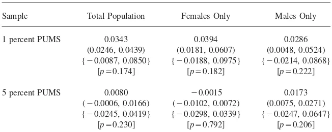
Table 3
Estimates for Merit Programs on Degree Attainment Using Person Weights, Adults Aged 22–34, 2000 PUMS
Coefficient Estimate on the Merit Aid Program Dummy Variable (Standard Cluster by State 95 Percent Confidence Interval)
{Conley and Taber 95 Percent Confidence Interval} [Cameron, Gelbach, and Miller Wild Cluster P-Value]
Sample Total Population Females Only Males Only
1 percent PUMS 0.0343 0.0394 0.0286
(0.0246, 0.0439) (0.0181, 0.0607) (0.0048, 0.0524) {ⳮ0.0087, 0.0850} {ⳮ0.0188, 0.0975} {ⳮ0.0214, 0.0868}
[p⳱0.174] [p⳱0.182] [p⳱0.222]
5 percent PUMS 0.0080 ⳮ0.0015 0.0173
(ⳮ0.0006, 0.0166) (ⳮ0.0102, 0.0072) (0.0075, 0.0271) {ⳮ0.0245, 0.0419} {ⳮ0.0298, 0.0339} {ⳮ0.0247, 0.0647}
[p⳱0.230] [p⳱0.792] [p⳱0.206]
Notes: Degree completion is defined as an associate’s or higher degree. All models include age and state of birth fixed effects and are weighted using the person weight variable.
results are the same (smallermeritcoefficients using the 5 percent PUMS than using the 1 percent PUMS, with most of the difference driven by females, but the differ-ences are not statistically significant).
The differences in means (both unweighted and weighted) between the 1 percent and 5 percent PUMS in Table 2 are often moderately large in magnitude for Ar-kansas, but are generally smaller for Georgia and for the rest of the United States. However, differences across samples are not statistically significant at conventional levels using a two-sample t-test except for the share of females that are nonwhite or Hispanic for the rest of the United States, which is significant at the 5 percent level.6 The significance here is an unexpected result and not easily explained. It
could be due to sampling error (if we examine enough variables, we might expect roughly 5 percent of them to have differences significant at the 5 percent level) or perhaps nonsampling error. Nonsampling error might arise because the Census does confidentially scrubs in which they alter individual records in the public use data in order to prevent individuals from being identifiable (U.S. Bureau of the Census 2003). For example, Alexander, Davern, and Stevenson (2010) show that nonsam-pling error in the 2000 PUMS results in very inaccurate age-specific gender ratios for persons age 65 and older.
We also calculate chi-square test statistics of whether the difference in means across the 1 percent and 5 percent PUMS are jointly zero for all five variables for
Arkansas and Georgia and all but the merit variable for the rest of the United States. None of the differences is statistically significant at the 5 percent level, but the differences for the rest of the United States are statistically significant at the 10 percent level.
Table 4 presents sample means for females by state of birth separately for persons ages 22–27 and 28–34 in Arkansas and the rest of the United States and ages 22– 25 and 26–34 in Georgia and the rest of the United States. The younger groups in Arkansas and Georgia are the ones exposed to the merit programs and the older groups and the rest of the United States are the controls. Again there are some differences between the unweighted and weighted means, and some differences be-tween the 1 percent and 5 percent PUMS. For brevity, we focus on the differences in weighted means between the 1 percent and 5 percent PUMS. The difference in the share of nonwhite or Hispanic is significant for the rest of the United States for ages 22–27 and ages 22–25, though we are again unsure why. More importantly for our purposes, the differences in the shares with an associate’s degree or higher are significant for Arkansans ages 28–34 and for Georgians ages 22–25. These differ-ences are driving the differdiffer-ences in themeritcoefficient between the 1 percent and 5 percent PUMS. However, it is not clear which sample is “correct”.
Table 4 also reports the chi-square test statistic for the age groups by state of birth. The test reports that the differences in means across the 1 percent and 5 percent PUMS for Georgians ages 22–25 are jointly significantly at the 5 percent level. Differences across the samples for all other groups in Table 4 are jointly insignificant except for the weighted means for the rest of the United States ages 22–27, which is significant at the 10 percent level. Finally, Table 5 reports means for the five constructed 1 percent subsamples. The chi-square test statistics report that the dif-ferences across the five 1 percent subsamples are not jointly statistically significant.
VII. Conclusion
States spend a substantial amount of money on aid programs, both need-based and merit. For example, in FY 2009, Georgia made 223,389 HOPE Scholarship awards and spent nearly $400 million. But we know very little about the effects of aid programs, particularly regarding their effects on college completion. Dynarski (2008) finds that the merit aid programs in Arkansas and Georgia increased college completion by about three percentage points.
282
The
Journal
of
Human
Resources
Table 4
Sample Means for Females by State of Birth and Age Group, 1 percent and 5 percent PUMS
State of Birth: Arkansas Rest of United States Georgia Rest of United States
Ages: 22–27 28–34 22–27 28–34 22–25 26–34 22–25 26–34
A. Unweighted Means 1 percent PUMS
Associate’s degree or higher 0.226 0.247 0.324 0.379 0.267 0.296 0.302 0.377 Bachelor’s degree or higher 0.167 0.186 0.241 0.285 0.193 0.226 0.221 0.284 Nonwhite or Hispanic 0.211 0.248 0.278 0.231 0.381 0.348 0.283 0.238 Living in birth state 0.647 0.641 0.690 0.652 0.756 0.740 0.698 0.657 5 percent PUMS
Sjoquist
and
W
inters
283
Associate’s degree or higher 0.246 0.265 0.339 0.394 0.288 0.313 0.317 0.392 Bachelor’s degree or higher 0.190 0.200 0.257 0.301 0.211 0.243 0.236 0.301 Nonwhite or Hispanic 0.236 0.276 0.290 0.248 0.389 0.347 0.294 0.255 Living in birth state 0.655 0.632 0.680 0.641 0.744 0.721 0.689 0.645 5 percent PUMS
Associate’s degree or higher 0.243 0.294* 0.340 0.394 0.250*** 0.321 0.316 0.393 Bachelor’s degree or higher 0.180 0.225 0.259 0.302 0.193 0.254 0.238 0.302 Nonwhite or Hispanic 0.266 0.273 0.286** 0.246 0.379 0.351 0.289** 0.252 Living in birth state 0.673 0.641 0.678 0.640 0.749 0.721 0.687 0.644 Chi-square test statistic 3.78 3.45 8.50 1.73 9.76 1.79 6.74 3.78 Chi-square test p-value 0.437 0.485 0.075 0.785 0.045 0.774 0.150 0.437
284 The Journal of Human Resources
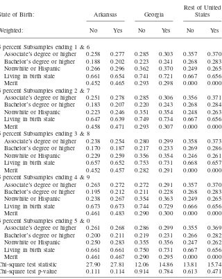
Table 5
Unweighted and Weighted Means for Females, Five 1 percent Subsamples
State of Birth: Arkansas Georgia
Rest of United States
Weighted: No Yes No Yes No Yes
5 percent Subsamples ending 1 & 6
Associate’s degree or higher 0.258 0.277 0.285 0.303 0.357 0.370 Bachelor’s degree or higher 0.188 0.202 0.223 0.241 0.268 0.283 Nonwhite or Hispanic 0.266 0.296 0.362 0.370 0.249 0.265 Living in birth state 0.661 0.654 0.741 0.721 0.667 0.656 Merit 0.452 0.465 0.293 0.298 0.000 0.000 5 percent Subsamples ending 2 & 7
Associate’s degree or higher 0.251 0.278 0.285 0.306 0.356 0.371 Bachelor’s degree or higher 0.183 0.207 0.220 0.243 0.268 0.284 Nonwhite or Hispanic 0.223 0.246 0.351 0.354 0.248 0.263 Living in birth state 0.647 0.639 0.749 0.734 0.667 0.656 Merit 0.458 0.471 0.293 0.307 0.000 0.000 5 percent Subsamples ending 3 & 8
Associate’s degree or higher 0.238 0.254 0.280 0.299 0.358 0.373 Bachelor’s degree or higher 0.170 0.187 0.217 0.233 0.269 0.286 Nonwhite or Hispanic 0.229 0.259 0.356 0.354 0.246 0.261 Living in birth state 0.657 0.652 0.753 0.731 0.668 0.657 Merit 0.452 0.457 0.282 0.291 0.000 0.000 5 percent Subsamples ending 4 & 9
Associate’s degree or higher 0.263 0.272 0.272 0.291 0.357 0.370 Bachelor’s degree or higher 0.195 0.212 0.211 0.228 0.268 0.283 Nonwhite or Hispanic 0.238 0.267 0.354 0.363 0.249 0.265 Living in birth state 0.673 0.673 0.744 0.729 0.666 0.656 Merit 0.461 0.483 0.290 0.300 0.000 0.000 5 percent Subsamples ending 5 & 0
Associate’s degree or higher 0.261 0.268 0.286 0.299 0.355 0.369 Bachelor’s degree or higher 0.200 0.211 0.219 0.231 0.266 0.282 Nonwhite or Hispanic 0.250 0.283 0.355 0.356 0.247 0.262 Living in birth state 0.661 0.661 0.750 0.731 0.667 0.656 Merit 0.461 0.467 0.290 0.295 0.000 0.000 Chi-square test statistic 27.90 27.81 12.06 14.86 13.81 15.74 Chi-square test p-value 0.111 0.114 0.914 0.784 0.613 0.471
References
Abadie, Alberto, Alexis Diamond, and Jens Hainmueller. 2010. “Synthetic Control Methods for Comparative Case Studies: Estimating the Effect of California’s Tobacco Control Program.”Journal of the American Statistical Association105(490): 493–505. Alexander, Trent, Michael Davern, and Betsey Stevenson. 2010. “Inaccurate Age and Sex
Data in the Census PUMS Files: Evidence and Implications.” Working Paper 15703. Cambridge: National Bureau of Economic Research.
Bell, Robert M., and Daniel F. McAffrey. 2002. “Bias Reduction in Standard Errors for Linear Regression with Multi-Stage Samples.”Survey Methodology28(2):169–81. Bertrand, Marianne, Esther Duflo, and Sendhil Mullainathan. 2004. “How Much Should We
Trust Differences-in-Differences Estimates?”Quarterly Journal of Economics119(1):249– 75.
Cameron, A. Colin, Jonah B. Gelbach, and Douglas L. Miller. 2008. “Bootstrap-Based Improvements for Inference with Clustered Errors.”Review of Economics and Statistics 90(3):414–27.
Conley, Timothy G., and Christopher R. Taber. 2011. “Inference with ‘Difference in Differences’ with a Small Number of Policy Changes.”Review of Economics and Statistics93(1):113–25.
Cornwell, Christopher, David B. Mustard, and Deepa J. Sridhar. 2006. “The Enrollment Effects of Merit-Based Financial Aid: Evidence from Georgia’s HOPE Program.”Journal of Labor Economics24(4):761–86.
Donald, Stephen G., and Kevin Lang. 2007. “Inference with Difference-in-Differences and Other Panel Data.”Review of Economics and Statistics89(2):221–33.
Dynarski, Susan. 2000. “Hope for Whom? Financial Aid for the Middle Class and Its Impact on College Attendance.”National Tax Journal Part 253(3):629–61.
———. 2004. “The New Merit Aid.” InCollege Choices: The Economics of Where to Go, When to Go, and How to Pay for It, ed. Caroline Hoxby, 63–97. Chicago: University of Chicago Press.
———. 2008. “Building the Stock of College-Educated Labor.”Journal of Human Resources43(3):576–610.
Henry, Gary T., Ross Rubenstein, and Daniel T. Bugler. 2004. “Is HOPE Enough? Impacts of Receiving and Losing Merit-Based Financial Aid.”Educational Policy18(5):686–709. MacKinnon, James, and Halbert White. 1985. “Some Heteroskedasticity-Consistent
Covariance Matrix Estimators with Improved Finite Sample Properties.”Journal of Econometrics29(3):305–25.
Ruggles, Steven, Matthew Sobek, Trent Alexander, Catherine Fitch, Ronald Goeken, Patricia Kelly Hall, Miriam King, and Chad Ronnander. 2008.Integrated Public Use Microdata Series: Version 4.0[Machine-readable database]. Minneapolis: Minnesota Population Center.