An Evaluation of Instrumental
Variable Strategies for Estimating
the Effects of Catholic Schooling
Joseph G. Altonji
Todd E. Elder
Christopher R. Taber
A B S T R A C T
Several previous studies have relied on religious affiliation and the proximity to Catholic schools as exogenous sources of variation for identifying the effect of Catholic schooling on a wide variety of outcomes. Using three sep-arate approaches, we examine the validity of these instrumental variables. We find that none of the candidate instruments is a useful source of identifi-cation in currently available data sets. We also investigate the role of exclu-sion restrictions versus nonlinearity as the source of identification in bivariate probit models. The analysis may be useful as a template for the assessment of instrumental variables strategies in other applications.
I. Introduction
The question of whether private schools, including Catholic schools, provide better education than public schools is at the center of the current national debate over the role of vouchers, charter schools, and other reforms that increase choice in education. All serious studies comparing Catholic and public schools
Joseph G. Altonji is a professor of economics at Yale University and a researcher with the National Bureau of Economic Research. Todd E. Elder is an assistant professor of economics and of labor and industrial relations at the University of Illinois at Urbana-Champaign. Christopher R. Taber is an associ-ate professor of economics at Northwestern University and a researcher with the National Bureau of Economic Research. This research was supported by the Institute for Policy Research, Northwestern University, the National Science Foundation under grant SBR 9512009, and the NIH-NICHD under grant R01 HD36480-03. The authors are grateful to Timothy Donohue for excellent research assistance and to Jeffrey Grogger, Derek Neal, and participants in seminars at Boston College, Michigan State University, Northwestern University, Purdue University, University College London, University of Missouri, University of Virginia, and University of Wisconsin for helpful comments. The authors claim responsibility for the remaining shortcomings of the paper. The data used in this article are confidential and can be obtained by special agreement with the National Center for Educational Statistics:
http://nces.ed.gov/pubsearch/licenses.asp
[Submitted December 2002; accepted February 2005]
ISSN 022-166X E-ISSN 1548-8004 © 2005 by the Board of Regents of the University of Wisconsin System
acknowledge the problem of nonrandom selection into Catholic schools and most wrestle with it in one way or another.1In the absence of experimental data, the main option is to find a nonexperimental source of variation Ziin Catholic school atten-dance that is exogenous with respect to the outcome under study. The problem, how-ever, is that most student background characteristics that influence schooling decisions, such as income, attitudes, and education of the parents, are likely to influ-ence outcomes independently of the school since they are likely to be related to other parental inputs. Characteristics of private and public schools such as tuition levels, student body characteristics and school policies are also poor candidates for excluded instruments because they are likely to be related to the effectiveness of the schools.
Two influential papers provide potential instrumental variables. Evans and Schwab (1995) treat Catholic schooling as exogenous in much of their analysis, but also pres-ent estimates that rely in part on the assumption that religious affiliation affects whether a person attends a Catholic school but has no independent effect on the out-come under study. Specifically, they use a dummy variable for affiliation with the Catholic church (Ci) as their excluded variable. Some support for this assumption is evidenced by the fact that Catholics are significantly more likely than non-Catholics to attend Catholic school, while Catholics are not far from national averages on many socioeconomic indicators. Evans and Schwab find a strong positive effect of Catholic school attendance on high school graduation and on the probability of starting col-lege. However, as Murnane (1985), Tyler (1994), and Neal (1997) note and as Evans and Schwab acknowledge, being Catholic could well be correlated with characteris-tics of the neighborhood and family that influence the effectiveness of schools.2
Neal (1997) uses proxies for geographic proximity to Catholic schools and subsi-dies for Catholic schools as exogenous sources of variation in Catholic high school attendance (see also Tyler 1994). The basic assumption is that the location of Catholics or Catholic schools was determined by historical circumstances unrelated to unobservables that influence performance in schools. Using data from the National Longitudinal Survey of Youth (NLSY), Neal estimates bivariate probit models of Catholic high school attendance and high school graduation in which Catholic school effects are identified by excluding whether the person is Catholic and either the frac-tion of Catholics in the county populafrac-tion in the case of urban minorities or the num-ber of Catholic schools per square mile in the county in the case of urban whites (Table 6, p. 113). His point estimates are not very sensitive to adding Catholic to the outcome equation.
The interaction between whether a person is Catholic and the availability of Catholic schools is a natural alternative to using distance or religion separately. It is
1. A few examples of early studies of Catholic schools and other private schools are Coleman et al (1982), Goldberger and Cain (1982), Alexander and Pallas (1985), Coleman and Hoffer (1987), and Bryk et al (1993). Recent studies include Evans and Schwab (1993,1995), Tyler (1994), Neal (1997), Figlio and Stone (1998), Grogger and Neal (2000), Sander (2001), and Jepsen (2003). Murnane (1984), Witte (1992), Chubb and Moe (1990), and Cookson (1993) provide overviews of the discussion and references to the literature. 2. Neal (1997) points out that one problem with using Cias an instrumental variable when estimating Catholic school effects (as in Neal, 1997, and Evans and Schwab, 1995) is that religious identification might be influenced by the school type attended. Neither study investigates the issue. In the case of NELS:88 we use the parent’s report of religious affiliation while the student is in eighth grade as our religion measure, but our results are not very sensitive to using the child’s tenth grade report instead.
possible that proximity to Catholic schools is related to differences in regional and family characteristics that have a direct influence on schooling and labor market out-comes, given that Catholic schools are somewhat concentrated by region.3However, since “tastes” for Catholic schooling depend strongly on religious preference, the interaction between distance (Di) and religious affiliation will have an effect on Catholic school attendance that is independent of the separate effects of religious affil-iation and distance. In particular, Catholic school attendance is likely to be much more sensitive to distance for Catholics than for non-Catholics. Consequently, one can con-trol for both religious affiliation and for distance from Catholic schools, as well as for a set of other geographic characteristics, while excluding the interaction Ci×Difrom outcome models. However, the case that Ci×Dimay be a valid instrument even if Ci and Diare not is far from bulletproof. Catholic parents who want their children to attend Catholic schools might choose to live near Catholic schools. This could lead to a positive or negative bias depending on the relationship between preferences for Catholic school and the error component in the outcome equation. Also, past immi-gration patterns and internal miimmi-gration from city to suburb and across regions may have led to differences between Catholics and non-Catholics in the correlation between proximity to Catholic schools and observed and unobserved components of family background.
In this paper we explore the validity of Catholic religion, proximity to Catholic schools, and the interaction between religion and proximity as exogenous sources of variation for identifying the effects of Catholic schooling on educational attainment and achievement. Our analysis may be of broader interest as a prototype for evalua-tions of instrumental variables strategies that could be conducted in other domains. Given that our conclusions are negative on the utility of the instruments, it is impor-tant to stress at the outset that the papers cited above recognize the potential problems with the exogeneity and power of the instruments that we investigate here. In partic-ular, Grogger and Neal (2000, p. 191) reach the conclusion that bivariate probit strate-gies are not very informative in the context of one of our main data sets—the National Educational Longitudinal Survey of 1988 (NELS:88).
We use multiple data sets and methods in our evaluation. In addition to the National Educational Longitudinal Survey of 1988 (NELS:88), we also report results based on the National Longitudinal Study of the High School Class of 1972 (NLS-72). For each instrument, we present 2SLS and bivariate probit estimates that rely on the particular instrument as the source of identification and compare the results to OLS and uni-variate probit estimates.
In addition to examining the a priori case for the instruments and the face plausi-bility and precision of the IV estimates, we assess the quality of the instruments in two other ways. The first takes advantage of the fact that few students who attend pub-lic eighth grades attend Cathopub-lic high school, regardless of religion or proximity. This provides some justification for using the coefficient on the instrument in a reduced-form outcome equation from a sample of public eighth grade attendees in NELS:88 as an estimate of the direct link between Catholic religion and the outcome. The second
3. Hoxby (1995) discusses geographical concentration by region, much of which is associated with the geo-graphic concentration of the Catholic population in the past.
approach uses a methodology introduced in Altonji, Elder and Taber (2002; hereafter, AET) to assess the instrumental variable results. AET’s approach is based on the prac-tice of using the degree of selection on observables as a guide to how much selection there is on unobservables.4
Finally, we investigate differences in the point estimates and standard errors obtained using 2SLS and bivariate probit and show that, at least in our data, religion and nonlinearities in the effects of religion and family background rather than the location variable instruments are the main sources of identification when we use Neal’s measures of proximity to Catholic schools.
In Section II we discuss the data from NLS-72 and NELS:88 that are used in the study. In Section III we present results using religion as the source of identification and provide some initial evidence on the direct effect of being Catholic on educational attain-ment. We also introduce and apply AET’s method of using the observables to assess the potential for bias due to an association between the instrument and the unobservables. In Section IV and in Section V we present results using distance and the interaction between distance and religion as the excluded instruments. In Section VI we investigate the role of exclusion restrictions versus nonlinearity as the source of identification in bivariate probit models. Section VII concludes with a research agenda.
II. Data
A. NELS:88
NELS:88 is a National Center for Education Statistics (NCES) survey that began in the Spring of 1988. A total of 1,032 schools contributed as many as 26 eighth grade students to the base year survey, resulting in 24,599 eighth graders participating. Subsamples of these individuals were reinterviewed in 1990, 1992, and 1994. The NCES only attempted to contact 20,062 base-year respondents in the first and second followups, and only 14,041 in the 1994 survey. Additional observations are lost due to attrition.
Parent, student, and teacher surveys in the base year provide information on family and individual background and on pre-high school achievement and behavior. Each student was also administered a series of cognitive tests in the 1988, 1990, and 1992 surveys to ascertain aptitude and achievement in math, science, reading, and history. We use standardized item response theory (IRT) test scores that account for the fact that the difficulty of the 10th and twelfth grade tests taken by a student depends on the eighth grade scores. We use the eighth grade test scores as control variables and the 10th and twelfth grade reading and math tests as outcome measures.
We calculate distance from the nearest Catholic high school as the distance from the zip code centroid of the respondent’s eighth grade school to the zip code centroid
4. Researchers often informally argue for the exogeneity of membership in a “treatment group” or of an instrumental variable by examining the relationship between group membership or the instrumental variable and a set of observed characteristics, or by assessing whether point estimates are sensitive to the inclusion of additional control variables. See for example, Currie and Duncan (1990), Engen et al (1996), Angrist and Evans (1998), Jacobsen et al. (1999), Bronars and Grogger (1994), and Udry (1998).
of the closest Catholic high school.5Our distance measure D
iis a vector of mutually exclusive indicators for distance less than one mile, one to three miles, three to six miles, six to 12 miles, and 12 to 20 miles, with greater than 20 miles treated as the omitted category. Our religion indicator Ciis one if parents indicated that they are Catholic in response to a question about religious affiliation in the base year survey and is zero otherwise.
Our main outcome measures are high school graduation (HSi) and college atten-dance (COLLi). HSiis one if the respondent graduated high school by the date of the 1994 survey, and zero otherwise.6COLL
iis one if the respondent was enrolled in a four-year university at the date of the 1994 survey and zero otherwise.7The indicator variable for Catholic high school attendance, CHi, equals one if the current or last school in which the respondent was enrolled was Catholic as of 1990 (two years after the eighth grade year) and zero otherwise.8 Unless noted otherwise, the results reported in the paper are weighted.9
B. NLS-72
The NLS-72 is a Department of Education survey of high school students that con-tains information on 22,652 persons who were seniors during the 1971–72 academic year. Additional interviews were conducted in 1973, 1974, 1976, 1979, and 1986. The final sample sizes are 19,489 students from 1,192 public high schools and 71 Catholic high schools for the college attendance indicator variable and 14,671 students from 879 public high schools and 57 Catholic high schools for the math and reading score variables.10
5. Detailed information on zip code characteristics of the eighth grade school (at the zip code level) is avail-able on the NELS:88 Restricted Use files. For the NELS:88 analysis, the zip code of every Catholic high school in the United States in 1988 was obtained from Ganley’s Catholic High Schools in America: 1988. The distance from a particular zip code centroid to the centroids of all the Catholic high schools was calcu-lated using an algorithm obtained from the U.S. National Oceanic and Atmospheric Administration. 6. We obtain similar results using a “drop out” dummy variable which equals one if a student dropped out of high school by 1992, or if the student dropped out of high school by 1990 and was not reinterviewed in 1992 or 1994, zero otherwise. This variable catches dropouts who left the survey by 1990 and were either dropped from the sample or were nonrespondents.
7. Our major findings are robust to whether or not college attendance is limited to 4-year universities, full-time versus part-full-time, or enrolled in college “at some full-time since high school” or at the survey date. 8. A student who started in a Catholic high school and transferred to a public school prior to the tenth grade survey would be coded as attending a public high school (CH = 0). If such transfers are frequently motivated by discipline problems, poor performance, or alienation from school, then misclassification of the transfers as public high school students could lead to upward bias in estimates of the effect of CHon educational attainment. AET present evidence that this issue is of minor importance.
9. The sampling scheme in the NELS:88 is explained in AET and Grogger and Neal (2000). The results are somewhat sensitive to the use of sample weights, although our main findings are robust to weighting. Given the choice based sampling scheme the weighted estimates are clearly preferred.
10. The 2,236 students who did not report their religious affiliation are excluded from the analysis. We also drop an additional 495 students for whom we could not impute distance from the nearest Catholic high school, reducing the sample size to 19,921. We also exclude 111 cases in which the student attended a non-Catholic private school, and additional observations are lost because data for key control variables and out-comes are missing.
The variable Ciis one for students who indicated they were Catholic in response to a base year question about religious affiliation and is zero otherwise. Distance from the nearest Catholic high school was recorded as the distance in air miles between the centroids of the zip code of residence reported in the first followup and the zip code of the nearest Catholic high school, and our distance measure Diis defined as a set of indicator variables identical to those used in the NELS:88 data.11The followup sur-vey included an indicator for whether the respondent had moved between their senior year of high school and the survey date, so the 10,530 students who moved were assigned the mean value of distance for all nonmovers who attended the same high school.12
In the original design, schools with a high percentage of minority students and in low-income areas are overrepresented, and sampling weights also vary with whether the school is public or private. The results are not sensitive to weighting procedures, and so we report unweighted estimates.
III. Using Religious Affiliation to Identify the Catholic
School Effect
In Table 1 we present univariate probit, OLS, bivariate probit, and 2SLS estimates of the Catholic school effect. The table footnotes provide a list of the family background, city size, student characteristic and eighth-grade behavioral and academic outcome variables that are included in both the equations for CHiand the outcomes (Yi). In this section our focus is on the first column, in which we use Cias the excluded instrument and include Dibut not Ci× Diin the equations for both CHi and Yi. Before proceeding further it is worth emphasizing that throughout the paper, we focus on homogenous treatment effects models, although in Section VI we esti-mate separate models for urban whites and urban minorities. In reality, the gains from Catholic school attendance probably vary with the quality of the local Catholic school and public school and the match between the student and the school. If one regards the estimates as local average treatment effects in the spirit of Imbens and Angrist (1994), one would expect some variation in estimates to arise across data sets.
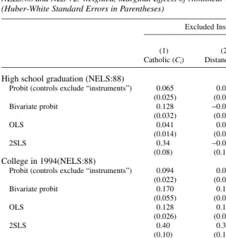
In NELS:88 the 2SLS estimate of the effect of CHion high school graduation is 0.34 (0.08). This estimate is unreasonably large given that the sample mean of HSiis 0.84. The bivariate probit estimate of the average marginal effect is a more reasonable value of 0.128 (0.032), but it is still double the univariate probit estimate. The esti-mates of the effect of CHion enrollment in a four-year college in 1994 are also inap-propriately large, as the 2SLS coefficient of 0.40 (0.10) is larger than the sample mean of 0.29. The bivariate probit estimate of 0.170 (0.055) is also well above the univari-ate probit estimunivari-ate of 0.094 (0.022).
11. The zip code of every Catholic high school in existence in the United States is listed in the U.S. Department of Education’s “Universe of Private Schools.”
12. The 495 students who were dropped because no distance measures could be created for them either attended one of the 26 high schools for which there are no valid observations on distance, or did not have valid values for the geographic move variable. These schools were part of NLS-72’s “backup sample,” and the students in this subsample were lost because they were excluded from the first followup.
We obtain a different pattern in NLS-72 (bottom panel). On one hand, the probit estimate of the effect of CHion college attendance is 0.068 (0.016), which reasonably close to the corresponding NELS:88 coefficient of 0.094. However, in NLS-72 the use
Altonji, Elder, and Taber 797
Table 1
Probit, Bivariate Probit, OLS, and 2SLS Estimates of Catholic Schooling Effects. NELS:88 and NLS-72. Weighted, Marginal Effects of Nonlinear Models Reported, (Huber-White Standard Errors in Parentheses)
Excluded Instruments
(1) (2) (3)
Catholic (Ci) Distance (Di) Ci×Di
High school graduation (NELS:88)
Probit (controls exclude “instruments”) 0.065 0.047 0.052
(0.025) (0.025) (0.026)
Bivariate probit 0.128 −0.007 −0.022
(0.032) (0.085) (0.119)
OLS 0.041 0.021 0.023
(0.014) (0.014) (0.015)
2SLS 0.34 −0.04 0.09
(0.08) (0.10) (0.11)
College in 1994(NELS:88)
Probit (controls exclude “instruments”) 0.094 0.085 0.077
(0.022) (0.022) (0.022)
Bivariate probit 0.170 0.103 −0.043
(0.055) (0.062) (0.070)
OLS 0.128 0.119 0.111
(0.026) (0.026) (0.026)
2SLS 0.40 0.31 −0.11
(0.10) (0.11) (0.12)
College in 1976 (NLS-72)
Probit (controls exclude “instruments”) 0.068 0.070 0.067
(0.016) (0.016) (0.016)
Bivariate probit −0.002 −0.052 −0.080
(0.028) (0.035) (0.035)
OLS 0.071 0.075 0.072
(0.015) (0.016) (0.016)
2SLS 0.06 0.44 −0.25
(0.04) (0.20) (0.11)
Notes
1. All models other than univariate probits OLS instrument for Catholic high school attendance (CHi).
2. Controls for all NELS:88 models include the demographic, family background, geography, and eighth grade variables listed in Table 3a. Controls for all NLS-72 models include the demographic, family back-ground, and geography variables listed in Table 3b. When Diis used as an instrument, Ciis included as a
control; when Ciis an instrument, Diis included; and when Di×Ciis an instrument, both Diand Ciare
included.
of 2SLS does not lead to a big increase in estimated effects. (The point estimate is 0.06, which is not significantly different from zero even though it implies a large effect, so the apparent similarity should be interpreted cautiously.) The NELS:88 results change very little when we condition the analysis on making it to twelfth grade or on HSi= 1, so we cannot attribute the similarity of the results from 2SLS and sin-gle-equation methods in NLS-72 but not NELS:88 to the fact that NLS-72 is limited to those who have made it to twelfth grade. We suspect that part of the difference in results for the two data sets is due to improvements over time in the relative social position of the Catholic population with school age children in the United States. The larger gap between the observed characteristics of Catholics and non-Catholics in NELS:88 relative to NLS-72 (Tables 3a and 3b) is consistent with this, as we discuss below. However, we do not have a full explanation.
The NLS-72 bivariate probit estimate is only −0.002, but it should be kept in mind that the source of identification in the bivariate probit case is a complicated nonlinear function of the variables in the model for CHiand not simply Ci, even though only Ci is excluded from the outcome equation. In particular, the analysis in Section VI below implies that the interaction between Ciand Diplays an important role in bivariate pro-bit and leads the bivariate propro-bit point estimate to be smaller than the 2SLS estimate. Our analysis suggests that identification of the bivariate probit comes primarily from the functional form assumptions rather than the exclusion restrictions in some cases. Thus, to assess the validity of the instruments, we focus on the 2SLS results.
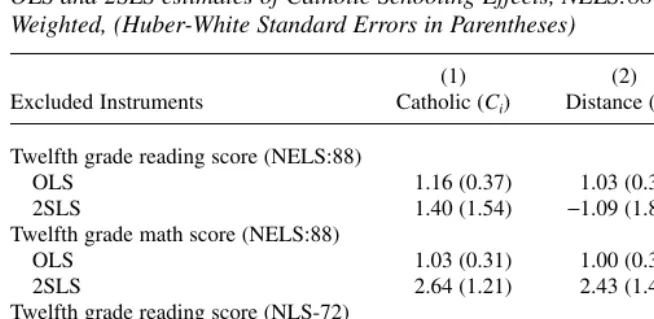
Table 2 reports OLS and 2SLS estimates of the effect of Catholic high school on test scores in NELS:88 and a variety of outcomes in NLS-72. Column 1 shows that the 2SLS estimates are larger for both NELS test scores than the single-equation ones, although the 2SLS coefficients are noisy. The standard deviation of these tests is 10, so the 2SLS estimate of 2.64 implies a large impact on twelfth grade math scores. However, the fact that the OLS estimates are uniformly smaller indicates that either 2SLS is biased upward or that Catholic high school students are actually negatively selected on the basis of unmeasured factors that are correlated with test scores. The NLS-72 test score results follow the opposite pattern—2SLS estimates are negative while OLS is large and positive for both reading and math. The NLS-72 analysis does not control for eighth grade achievement, but this disparity does not account for the differences in patterns between the two data sets, as (unreported) NELS:88 models that do not control for eighth grade achievement generate similar results to the NELS:88 models in Table 2.
To summarize, in NELS:88 the 2SLS estimates using Cias the excluded instrument imply that the Catholic school effect is very large, particularly for educational attain-ment. The NLS-72 results are more mixed but are consistent with a substantial posi-tive effect on educational attainment. One might be tempted to conclude that the IV estimates, while unreasonably large, bolster the probit and OLS evidence that the true effect is substantial. In the remainder of this section, we argue that this is the wrong interpretation.
A. Comparing Catholics and Non-Catholics on the Basis of Observables
Column 1 of Table 3a presents sample means of a set of family background charac-teristics, student characcharac-teristics, eighth grade outcomes, and high school outcomes in The Journal of Human Resources
NELS:88, and Column 2 shows the difference between Catholics and non-Catholics in these means.13 Catholics are 7 percentage points more likely to graduate high school and 8 percentage points more likely to be enrolled in a four year college in 1994. Differences in tenth and twelfth grade test scores are more modest but all show a significant advantage for Catholic students. If Catholic was as good as randomly assigned, these differences would be entirely attributed to the fact that Catholics are more likely to attend Catholic high school. It would then be troubling if Catholic appeared to be related to a broad set of variables determined prior to high school enrollment that influence high school outcomes. Consequently, we begin our evalua-tion of Catholic religion as an excluded instrument by following the common practice of simply comparing the characteristics of Catholics and non-Catholics in both NELS:88 and NLS-72.
Differences by Ciappear in many of the family and student characteristics and eighth grade outcomes in Table 3a. There is a modest positive association between Catholic religion and parental educational expectations, with a gap of 0.04 in the fraction of par-ents who expect their children to attend some college and 0.03 in the fraction who
13. In Table 3a the outcome variables are weighted with the same weights used in the regression analysis, so that the tenth and twelfth grade test scores are weighted using first and second followup panel weights, respectively, and high school graduation and college attendance are weighted by third followup weights. All other variables are weighted using second followup panel weights.
Altonji, Elder, and Taber 799
Table 2
OLS and 2SLS estimates of Catholic Schooling Effects, NELS:88 and NLS-72, Weighted, (Huber-White Standard Errors in Parentheses)
(1) (2) (3)
Excluded Instruments Catholic (Ci) Distance (Di) (Ci×Di)
Twelfth grade reading score (NELS:88)
OLS 1.16 (0.37) 1.03 (0.37) 1.14 (0.38)
2SLS 1.40 (1.54) −1.09 (1.84) 1.24 (1.82)
Twelfth grade math score (NELS:88)
OLS 1.03 (0.31) 1.00 (0.31) 0.92 (0.32)
2SLS 2.64 (1.21) 2.43 (1.45) −2.63 (1.57)
Twelfth grade reading score (NLS-72)
OLS 2.06 (0.34) 2.54 (0.37) 2.50 (0.36)
2SLS −1.34 (0.99) 8.69 (4.53) 0.50 (2.32)
Twelfth grade math score (NLS-72)
OLS 1.52 (0.33) 1.77 (0.35) 1.71 (0.36)
2SLS −0.07 (0.96) 11.05 (4.47) −3.94 (2.27)
Notes:
1. All 2SLS models instrument for Catholic high school attendance (CHi).
2. Controls for all models include those described in notes to Table 1. When Diis used as an instrument, Ci
is included as a control; when Ciis an instrument, Diis included; and when Di×Ciis an instrument, both Di
and Ciare included as controls.
The Journal of Human Resources
800
Table 3a
Comparison of Means of Key Variables by Value of Distance, Catholic, and their Interaction. NELS:88
(1) (2) (3) (4)
Overall Mean Difference by Ci Difference by Di Differenceby Ci×Di
Demographics
Female 0.50 0.01 0.00 0.00
Asian 0.04 0.01 0.04 −0.02
Hispanic 0.10 0.19 0.08 0.03
Black 0.13 −0.15 0.08 −0.13
White 0.73 −0.05 −0.20 0.12
Family background
Mother’s education 13.14 −0.26 0.17 −0.36
Father’s education 13.42 −0.07 0.17 −0.31
Log of family income 10.20 0.11 0.12 −0.02
Mother only in house 0.15 −0.04 0.02 −0.03
Parent married 0.78 0.06 −0.02 0.03
Geography
Rural 0.32 −0.15 −0.44 0.05
Suburban 0.44 0.06 0.08 0.00
Urban 0.24 0.09 0.36 −0.05
Expectations
Schooling 15.17 0.15 0.31 −0.06
Very sure to graduate high school 0.83 −0.01 0.00 −0.01
Parents: some college 0.88 0.04 0.05 −0.02
Parents: college graduates 0.88 0.03 0.06 −0.04
Altonji, Elder
, and T
aber
801
Eighth grade variables
Delinquency index 0.69 −0.05 0.03 −0.04
Got into fight 0.27 −0.01 0.01 0.05
Rarely do homework 0.21 −0.05 0.00 0.00
Frequently disruptive 0.13 −0.02 −0.01 0.00
Repeated grade 4–8 0.08 −0.03 0.01 −0.03
Risk index 0.72 −0.07 −0.01 0.01
Grades composite 2.89 0.04 0.00 0.07
Unprepared index 10.82 0.00 0.08 −0.09
Eighth grade reading 50.32 0.40 0.03 1.15
Eighth grade math 50.33 0.55 0.45 0.06
Outcomes
Tenth grade reading 50.16 0.65 0.58 0.60
Tenth grade math 50.21 0.93 0.75 −0.50
Twelfth grade reading 50.40 0.52 0.88 −0.17
Twelfth grade math 50.38 1.18 1.03 −0.70
College in 1994 0.29 0.08 0.08 −0.05
High school graduate 0.84 0.07 0.01 0.01
Attended Catholic high school 0.06 0.13 0.12 0.15
Notes:
The Journal of Human Resources
802
Table 3b
Comparison of Means of Key Variables by Value of Distance, Catholic, and their Interaction. NLS-72
(1) (2) (3) (4)
Overall Mean Difference by Ci Difference by Di Difference by Ci×Di
Demographics
Female 0.50 −0.01 0.03 0.03
Hispanic 0.04 0.11 0.01 −0.07
Black 0.15 −0.15 0.04 −0.08
Family background
Mother’s education 12.19 −0.13 0.16 −0.33
Father’s education 12.43 0.06 0.40 −0.32
Log of family income 8.93 0.07 0.11 −0.03
Father blue collar 0.24 0.01 −0.03 −0.01
Low SES indicator 0.29 −0.05 −0.06 0.00
English language 0.92 −0.06 −0.02 0.03
Family gets paper 0.88 0.04 0.06 0.01
Altonji, Elder
, and T
aber
803
Geography
Rural 0.23 −0.14 −0.30 0.05
Suburban 0.48 0.06 0.02 −0.04
Urban 0.29 0.08 0.28 −0.01
Expectation
Decided on college prehigh school 0.41 −0.01 0.04 −0.06
Outcomes
College by 1976 0.38 0.01 0.05 −0.06
Reading score 50.01 0.30 0.46 0.55
Math score 49.98 0.58 0.40 −0.10
Years of PSE, 1979 1.61 0.03 0.22 −0.23
Attended Catholic high school 0.06 0.19 0.07 0.15
Notes:
The Journal of Human Resources 804
expect at least a college degree.14While the differential in family income is positive, it is negative in mother’s and father’s education. However, Table 3a also shows that Catholic students are favored across a broad set of measures available in eighth grade, such as test scores, grades, and teacher evaluations of the student’s behavior. Among these eighth grade variables, only the “unpreparedness index” variable does not vary favorably with Ci. The discrepancy in the fraction of students who repeated a grade in grades 4–8 is −0.03, and the gap in the fraction of students who are frequently disrup-tive is −0.02. The existence of gaps in favor of Catholic students across several dimen-sions suggests that Catholic and non-Catholic students differ in many respects, some of which may be unobservable to empirical researchers. Since these differences also con-tribute to high school and post-high school outcomes (see AET for evidence), doubts arise regarding the validity of using Cias an instrumental variable for Catholic high school attendance.
In NLS-72, the differences are less pronounced, although it appears that overall Catholic religion has a weak positive association with favorable family background characteristics. Log family income is 0.07 higher for Catholics, who are also five per-centage points less likely to be members of families which meet NLS-72’s definition of low socioeconomic status. There are essentially no differences in parental educa-tion levels or pre-high school student educaeduca-tional expectaeduca-tions.
Given the overall picture of Tables 3a and 3b, we anticipate that the use of Cias an instrumental variable will likely result in positively biased estimates of Catholic schooling effects in NELS:88 and perhaps a small positive bias in NLS-72, although it is difficult to gauge its extent. The richness of the NELS:88 data permits us to use two more formal procedures to gauge the magnitude and direction of the bias.
B. The Effect of Catholic Religion for Students from Public Eighth Grades
One way to assess the endogeneity of Catholic religion is to identify a sample of per-sons for whom Catholic high school is not a serious option, and then interpret the coefficient on Ci in a single equation model as an estimate of the direct effect of Catholic religion on the outcome. Public eighth graders provide such a sample, because only 0.3 percent of public school eighth graders in our effective sample go on to attend Catholic high school, with the percentage being only 0.7 percent even among public eighth grade attendees whose parents are Catholic.
Let the outcome Yibe determined by (1) Yi= αCHi+ Xilγ + εi,
where γis defined so that cov(εi, Xi) = 0. CHiis potentially endogenous and thus cor-related with εi. We assume that our instrument Cidoes not influence Yidirectly but is correlated with CHi. However, there is concern that Ciis correlated with εi.
Define β, π, and λto be the coefficients of the least squares projections
(2) proj(Ci⎪Xi) = Xil π,
(3) proj(CHi⎪Xi, Ci) =Xilβ + λCi.
Define C~ias the residual of the projection of Cion Xiso that
(4) C~i ≡ Ci– Xilπ.
It is well known that the IV estimate of αconverges to
(5) p piis attendance of a public eighth grade by individual i. We assume for now that the joint distribution of (Xi, Ci, εi) is independent of pi, but argue at the end of the section that accounting for correlation between Ciand εiinduced by restricting the analysis to the public eighth-grade sample is likely to strengthen the evidence against Cias an instrument.
Consider a regression of Yion Xiand Ciconditional on pi. Under these conditions, the coefficient on Ciwill converge to cov(Cui,fi)/var(Cui). Since we have a consistent estimate of λfrom the first stage regression, we can obtain a consistent estimate of the bias }=cov(Cui,fi)/(mvar(Cui)) by estimating the parameter ψ in the regression model
(6) Yi=XliK+[Cu tim }] +~i
on the public eighth grade sample.
In Column 1 of Table 4 we report estimates of the bias parameter ψ using this approach to evaluate Catholic religion as an instrument.15We present separate equa-tions estimated for HSi, COLLi, and the twelfth grade math and reading test scores. The vector Xiincludes all of the other controls that were included in our models in Tables 1 and 2. For ease of comparison, the table also presents the corresponding 2SLS estimates from Table 1 and 2.
The results are striking—the implied bias in the 2SLS estimate is 0.34 (0.08) for HSi, which is identical to the 2SLS coefficient itself.16The large potential bias should raise a great deal of concern about using Catholic as an instrument, particularly given the remarkable similarity between the magnitudes of the bias and the 2SLS estimate. In our view, this evidence alone is sufficient to rule out Catholic religion as a useful instrument.
In the college attendance case the (unreported) estimate of cov(Cui,fi)/var(Cui)is 0.038 (0.013), indicating that Catholic students are nearly four percentage points
Altonji, Elder, and Taber 805
15. Eliminating the 36 students who attended public eighth grade and went on to Catholic high school makes little difference.
16. To see how we arrive at this figure, note that the estimate of cov(Ci,εi)/var(Ci) in the high school
The Journal of Human Resources
806
Table 4
Comparison of 2SLS Estimatesaand Bias Implied by OLS Estimation of Y
i= Xi′γ +[Zi′mt]ψ + ωi , on the Public Eighth Grade Subsample.bVarious Outcomes and instruments. NELS:88 Sample Weighted, (Huber-White Standard Errors in Parentheses)
Instruments (Zi)
Outcome (Y) (1) (2) (3)
Catholic Distance Catholic ×Distance
High school graduation
Implied bias in 2SLS (ψ)c 0.34 (0.08) −0.05 (0.12) 0.15 (0.12)
2SLS coefficient 0.34 (0.08) −0.04 (0.10) 0.09 (0.11)
College attendance
Implied bias in 2SLS (ψ) 0.29 (0.11) 0.37 (0.12) −0.23 (0.13)
2SLS coefficient 0.40 (0.10) 0.31 (0.11) −0.11 (0.12)
Twelfth Grade Reading Score
Implied bias in 2SLS (ψ) 0.54 (1.68) −0.51 (2.08) −0.50 (1.99)
2SLS Coefficient 1.40 (1.54) −1.09 (1.84) 1.24 (1.82)
Twelfth grade math score
Implied bias in 2SLS (ψ) 1.85 (1.41) 1.83 (1.69) −4.37 (2.06)
2SLS Coefficient 2.64 (1.41) 2.43 (1.45) −2.63 (1.57)
Notes:
a. Controls for all models include those described in notes to Table 1. In Column 1, Diis included as a control; in Column 2, Ciis included as a control; and in Column 3,
both Diand Ciare included as controls.
b. The model Yi= Xi′γ +[Zi′mt]ψ + ωi, is estimated by OLS using the NELS:88 sample of those who attended public eighth grade schools. Sample sizes: N = 7,701 (HS
Graduation), N = 7,481 (college attendance), N = 7,377 (twelfth reading), N = 7,380 (twelfth math). λis the coefficient on Ziin the first stage equation for CHi. The
sam-ple sizes for the first stage equations are listed in Tables 1 and 2 for the various outcomes. The 2SLS coefficients are from Tables 1 and 2.
more likely to enroll in a four year college than non-Catholics even when Catholic high school is not a serious option. This relationship implies a bias of 0.29 (0.11) in 2SLS estimates, so it seems likely that the large 2SLS estimates in Table 1 result from the endogeneity of Ciwith respect to both high school graduation and college atten-dance. Similar calculations suggest that the math test score estimate from Table 2 can largely be explained by potential bias of 1.85 (1.41) for the twelfth grade math scores. Part of the college attendance and test score effects may be “real,” as these large cor-rections are still smaller than the 2SLS point estimates, but the substantial evidence of endogeneity of Cicombined with the imprecision of the estimates prevents any firm conclusions about the effect of Catholic high school on these outcomes.
A selection problem arises because we are focusing only on public eighth graders. The analysis in this section has treated public eighth grade attendance as if it were randomly assigned. We would expect positive selection of Catholics into Catholic grade schools because it is costly and requires parental initiative and because we observe positive selection on a broad list of characteristics that raise school outcomes. That is, Catholic students who attend Catholic grade schools are likely to have higher values of εiin Equation 1 than Catholic students who attend public grade schools. Since non-Catholics are much less likely to attend Catholic schools this effect will lead to a negative bias in Cov C(ui,fi) when we condition on public school atten-dance.17This would imply that our estimates of ψare biased downward, which makes the results in this section even more surprising. However, while we believe that the above scenario is the most likely one, one could envision a Roy (1951) model of com-parative advantage in which children who gain less from attending a Catholic eighth grade school and high school conditional on the observables are more likely to attend public eighth grade school, or a model in which the children of parents who substi-tute between school and parental inputs when Catholic school is expensive relative to the cost of increasing parental inputs may be more likely to attend a public school.18 In either case, Catholic children may outperform non-Catholic children conditional on public eighth grade attendance even when Ciis a valid instrument.
C. Using the Observables to Assess the Bias from Unobservables
In this section we extend the methodology of AET to assess the potential bias in the instrumental variables estimates in Equation 1. AET consider the case in which an instrument (such as Ci) is not necessarily valid, and the researcher does not have a strong prior about how it is determined. In particular, rather than assume that the choice of Xiensures that Cuiis uncorrelated with εi, as is required for consistency of 2SLS, AET develop a model of data collection which implies that the effect on Ciof a unit change in the index of observables Xilγthat determine Yiis the same as the effect on Ciof a unit change in the index of unobservables εi. When the instrument is an indicator variable such as Ci, the condition may be written as
Altonji, Elder, and Taber 807
17. To see this in a simple case, abstract from observables so that Cui= Ci, and assume that non-Catholics
do not attend Catholic schools, that E(εi⎪Ci) = 0 unconditional on pi, and that there is positive selection into
Catholic eighth grades so that E(εi⎪Ci= 1, pic) > E(εi⎪Ci= 1, pi), where picis the complement of pi. This
implies that E(εi⎪Ci= 1, pi) < 0 and thus the bias is negative.
The Journal of Human Resources
the index of observables in the outcome equation that is associated with Ci, while the term [ ( |E fi Ci=1)-E( |fi Ci=0)]/Var( )fi is the corresponding normalized shift in
the distribution of unobservables. Using [ (E Xilc|Ci=1)-E X( ilc|Ci=0)]/Var(Xilc)
to assess the possibility that [ ( |E fi Ci=1)-E( |fi Ci=0)]/Var( )fi is substantially
different from zero is a formalization of the common practice of checking for a sys-tematic relationship between an instrumental variable and each of the elements of Xi, as we performed in Section IIIA above. Intuitively, if one estimates
i i
[ (E Xlic|Ci=1)-E X( lc|Ci=0)]/Var(Xlc)and finds that it is substantially different from zero, one may be worried that the null hypothesis E(εi⎪Ci) = 0 is wrong. The pre-cise assumptions that generate the above Condition are given in AET.
We can use Equation 7 to approximate the amount of bias in 2SLS estimates of Catholic schooling effects if selection on unobservables is similar to selection on observ-ables. It is straightforward to show that the asymptotic bias from 2SLS would be (8)
where we have used Equation 7 to obtain Equation 9 from Equation 8. The hypothe-sis of equal selection on observables and unobservables provides a way of identifying [E(εi⎪Ci= 1)–E(εi⎪Ci= 0)], and therefore the asymptotic bias of instrumental vari-able estimates, since the other terms in Equation 9 are readily and consistently estimable. AET develops extensions to the case of latent dependent variables, so both probit and linear 2SLS bias calculations are given where appropriate.
One should not make too much of the specific estimates of bias, which are based on strong assumptions about the symmetry of selection of observables and unobserv-ables. In AET, we argue that the relationship between the indices of unobservables that determine CHiand Yiis likely to be weaker than the relationship between the indexes of observables, in part because many of the factors that determine graduation and college attendance are determined after eighth grade and are excluded from Xiby design. We are less clear about the force of this argument in the case of Ciand the other instruments we consider. The variables Ci, Di, and Ci×Dicould all be correlated with pre- and post-eighth grade influences on Yithat are not correlated with CHi, but these correlations could be stronger or weaker than the link between factors that deter-mine CHi and Yi. However, we suspect that they are considerably weaker, which means that bias estimates will be too large in absolute value.
One may refine the bias calculations to account for the fact that the variation in the instrument may only be over a specific dimension. For example, Dionly varies across zip code, and so must be orthogonal to variation in Xliγand in εithat is within zip code. Consequently, we adjust the bias estimates by using variance in E(Xilγ) across
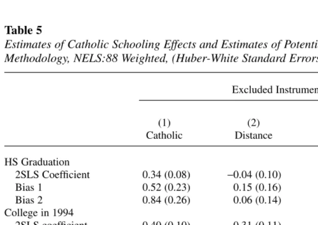
Column 1 of Table 5 presents the results, which are quite striking. In the case of high school graduation, for linear 2SLS we calculate a bias of 0.52 (0.23) in at if we include Diamong the set of variables used to form the index of observables and 0.84 (0.26) if we exclude it. These are both huge potential biases, greater in magnitude than the implausibly large 2SLS point estimate that is repeated in this table for conven-ience. In the case of COLL the bias estimate under the assumptions leading to Equation 7 is 0.45 (0.21), which is slightly larger than the 2SLS estimate of 0.40. If selection on unobservables follows the same pattern as selection on observables, there is a huge bias in the IV estimates when Ciis used as an instrument, at least for the cohort of children sampled in NELS:88.19The results reinforce our conclusions based on the public eighth grade sample. However, the bias estimates have large standard errors and are best interpreted as a sign of potential trouble rather than a precise esti-mate of the extent of the bias.
Altonji, Elder, and Taber 809
19. This conclusion is also supported by calculations not reported that use a two stage probit procedure. See Elder (2002) for details.
Table 5
Estimates of Catholic Schooling Effects and Estimates of Potential Bias Using AET Methodology, NELS:88 Weighted, (Huber-White Standard Errors in Parentheses)
Excluded Instruments
(1) (2) (3)
Catholic Distance Catholic ×Distance
HS Graduation
2SLS Coefficient 0.34 (0.08) −0.04 (0.10) 0.09 (0.11)
Bias 1 0.52 (0.23) 0.15 (0.16) 0.14 (0.24)
Bias 2 0.84 (0.26) 0.06 (0.14) —
College in 1994
2SLS coefficient 0.40 (0.10) 0.31 (0.11) −0.11 (0.12)
Bias 1 0.45 (0.21) 0.46 (0.22) 0.15 (0.26)
Bias 2 0.45 (0.21) 0.40 (0.20) —
Twelfth reading score
2SLS Coefficient 1.40 (1.54) −1.09 (1.84) 1.24 (1.82)
Bias 1 1.18 (1.06) 2.49 (1.59) 2.59 (1.14)
Bias 2 1.42 (1.07) 2.11 (1.40) —
Twelfth math score
2SLS Coefficient 2.64 (1.21) 2.43 (1.45) −2.63 (1.57)
Bias 1 2.02 (0.75) 1.76 (1.03) 1.42 (0.88)
Bias 2 1.87 (0.74) 1.72 (0.98) —
Notes:
1. Controls included are described in Table 1 notes.
2. Sample sizes: N = 8,560 (HS Graduation), N = 8,313 (College Attendance in NELS), N = 8,166 (twelfth reading), N = 8,199 (twelfth math).
3. “Bias 1” calculations use all variables, while “Bias 2” excludes Diand Ciin the bias calculations.
The bottom panels of Table 5 repeat the calculations for twelfth grade test scores. These calculations use estimates of the reliability of the NELS:88 tests to provide a rough adjustment for the fact that much of the variance in εiis due to noise in the tests and thus is unrelated to Ci.20The calculations suggest that there is the potential for substantial bias when using Cias an instrument, but the estimates are very imprecise. In the case of math the bias estimates of 2.02 (0.75) and 1.87 (0.74) (depending again on whether Diis used in the calculations) preclude any firm conclusions. In general, we cannot rule out the possibility of a positive effect of Catholic high school atten-dance on achievement test scores, but the large potential biases are suggestive that the use of Ci as an instrument is not a reliable way to assess the magnitude of these effects.
D. Summary of CiResults
All three approaches that we have used draw attention to potential problems with the use of Cias an instrument. It seems closely related to observable covariates, which causes one to be worried that it may produce bias. We then estimate the bias in two very different ways, both of which suggest that the estimates may be substantially positively biased. We conclude from these calculations that IV procedures based on Cilead to huge point estimates, but that Ciis not a useful instrumental variable despite its powerful association with CHi.
We have already noted that we do not fully understand why the gaps between IV and univariate estimates of the Catholic school effect are so much larger in NELS:88 than in NLS-72 or in High School and Beyond (See Evans and Schwab 1995). Unfortunately, we lack the rich set of primary school data required to use the relative degree of selection on observables to explore the discrepancy in IV results across data sets. The variability across data sets, which in part may reflect changes over time in the composition of the Catholic population in the United States, is an additional rea-son to be cautious about the use of Cias an instrument.
IV. Instrumental Variables Estimates using Proximity
to Catholic Schools
In this section we evaluate proximity (Di) as a source of identifying variation. In Column 2 of Table 1 we report estimates with Dias the excluded instru-ment, and again we focus on linear 2SLS because of concerns that functional form The Journal of Human Resources
810
20. The adjustment is performed by multiplying the estimate of plim (at-a)based on Equation 8 by (reliability–R2)/(1–R2), where reliabilityis the estimate of the reliability of the particular test, and R2is the
R2of the model for the particular test. To see the justification, let the composite error term be ε*= ε + ςwhere
ςis the component of test scores due to noise in the test. One minus the reliability of the test is an estimate of var(ς)/var(Yi+ ς) where Yiis the true test score. The value 1 minus the R2of the test score model is an
estimate of [var(ε) + var(ς)]/var(Yi+ ς), and note that since var(ε) = [var(ε)/(var(ε) + var(ς))]var(ε*),
*)/(1 -R )
( ) [( ) ( )] (
var f = 1+R2 - 1-reliability var f 2 . The R2is 0.60 for twelfth grade reading and
0.74 for twelfth grade math (using the 2SLS estimate of the model and ignoring the correlation between CHi
and εi), and the reliability is 0.85 for twelfth grade reading and 0.94 for twelfth grade math. Consequently,
assumptions are driving identification in bivariate probit models. The 2SLS esti-mate of −0.04 (0.10) for high school graduation is too imprecise for us to draw any inferences from it. The 2SLS estimates for COLLiare 0.31 (0.11) in NELS:88 and 0.44 (0.20) in NLS-72. Both estimates are much larger than the estimated marginal effects of 0.085 from the univariate probit in NELS:88 and 0.070 from NLS-72. Column 2 of Table 2 presents the results for test scores in NELS:88 and NLS-72. These coefficients vary across specifications, but for the NLS-72 test scores they imply very large effects. On their face, the findings for COLLand the NLS-72 test score results appear implausible. In the remainder of this section we look for evi-dence of bias.
In Column 3 of Table 3a we report the relationship between a wide set of observ-ables in NELS:88 and a student’s distance from the nearest Catholic high school. For simplicity we collapsed the vector Diinto a dummy variable D6i, which is equal to 1 for person iif she lives fewer than six miles from the nearest Catholic high school and zero otherwise, and present the difference in these means by D6i. Among the eighth grade measures, such as teacher evaluations of the student’s behavior, there is little difference between those who live close to Catholic high schools and those who do not. However, there is a positive relationship between D6iand most of the family background measures. There is also a positive association between proximity and both student and parental educational expectations. Similar differences by D6iappear in NLS-72 (Table 3b). These differences in family motivation and students’ home environment introduce the possibility that there might also be unmeasured differences which could affect outcomes and lead to bias in models using Dias an instrumental variable in both NLS-72 and NELS:88.
In Column 2 of Table 4 we report estimates of the bias coefficient ψbased on the equation
(10) Yi=Xlic+[Dl tim }] +~i
The results are in Column 2 of Table 5. The estimates computed under the assump-tion of equal selecassump-tion on observables and unobservables show the potential for large positive biases for both HSiand COLLi.The fact that the bias estimates for the two different outcomes have the same sign is not surprising, since it reflects the similarity in the effects of Xion the two education outcomes. While the specific bias estimates are noisy and are probably overstated for reasons discussed above, the large estimate for COLLisuggests that the 2SLS coefficients are not informative. Finally, for twelfth grade math scores, the estimates of 1.72–1.76 (depending on whether Ciis included in the calculations involving Xilc)again do not preclude a small Catholic schooling effect, but given both the evidence of endogeneity and the large standard errors of the 2SLS estimates, we conclude that the 2SLS estimates using Diare also not useful in drawing conclusions regarding test scores.21
V. Instrumental Variables Estimates Using
Catholic
¥
Distance
Finally, we turn to the interaction between Ciand Dias the source of identifying variation. All of the models include both Ciand Diamong the controls. In Column 3 of Table 1 we report probit, bivariate probit, linear probability, and 2SLS estimates of the effect of CHion high school graduation and college attendance. The bivariate probit and 2SLS point estimates are negative in two of the three cases. Column 3 of Table 2 presents results for test scores. The 2SLS estimates lie below the OLS ones in three of the four cases, with twelfth grade math score coefficients being fairly large and negative in both data sets. However, in all cases in NELS:88 the stan-dard errors are too large in relation to the difference between the OLS and 2SLS esti-mates for the 2SLS estiesti-mates to help much in modifying conclusions about α. This is less true in the NLS-72.
We have investigated the properties of the instrument using the same set of proce-dures that we used for Ciand Diwith the same bottom line. Given the imprecision in some of the estimates and space considerations, we will skip the details.22However, the weight of the evidence in Tables 1–5 leads us to be very skeptical of the interac-tion as an exclusion restricinterac-tion. In particular, there is evidence in both data sets that the difference between Catholics and non-Catholics in favorable family background characteristics rises with distance from the nearest Catholic high school. If the link between Ci×Diand εifollowed the same pattern, the 2SLS estimates would be biased The Journal of Human Resources
812
21. The public eighth grade analysis is probably less informative for Dithan for Cibecause of the likelihood
that distance from Catholic elementary school and distance from Catholic high school are closely related. Consequently, selection issues may have a bigger effect on the coefficient on the index when the distance variables are involved than when only religion is involved.
22. In Column 4 of Table 3a we report the coefficient on Ci×D6ifrom regressions of the various background
and outcome variables indicated in the rows on Ci,Di,and Ci×Di. The results for the eighth grade
meas-ures are mixed, with Ci×Dibeing positively associated with indicators for whether the student got into a
fight at school, but negatively correlated with the “repeated grade” indicator. There are also slight compara-tive advantages in eighth grade GPA and reading scores. In contrast, family background, student expecta-tions, and parental expectations are generally negatively correlated with Ci×Di, with striking differences in
downward. We suspect that this underlies the negative coefficients for some outcomes in both data sets, particularly NLS-72. We conclude that Ci×Diis not a very useful source of variation for the purpose of estimating the Catholic school effect, at least not in the context of NELS:88 or NLS-72.
VI. Exclusion Restrictions or Nonlinearity as the
Source of Identification? A Comparison
of Bivariate Probit and 2SLS
Thus far we have focused on whether the instruments are uncorrelated with the error components. In this section we focus on the power of the instruments for identification in nonlinear models. Both Evans and Schwab (1995) and Neal (1997) apply bivariate probits of Catholic schooling and educational attainment using data from High School and Beyond and NLSY, respectively. Both papers emphasize the importance of an exclusion restriction in the model for identification. As we have already noted, Evans and Schwab (1995) primarily rely on Catholic religion, exclud-ing it from the outcome equation but includexclud-ing it in the Catholic schoolexclud-ing decision. Neal (1997) uses an indicator for Catholic religion along with county level measures of Catholic church adherents as a fraction of county population (%CCHi) in the case of minorities and Catholic religion and Catholic secondary schools per square mile (CH/Mi) in the county in the case of whites. Both of these papers report positive effects of CHion educational attainment that are estimated fairly precisely, although Evans and Schwab (1995) experiment with 2SLS and obtain implausible results in some specifications.23Our bivariate probit results generally follow the same pattern, with estimates being much more precise and reasonable than linear specifications. It is therefore worth investigating the reasons why our instrumental variables results are so noisy and in many cases seem unreasonable, while the bivariate probits tend to gen-erate plausible, precise estimates.
Altonji, Elder, and Taber 813
For NLS-72, the estimates in Table 3b imply that the difference in mother’s and father’s education between Catholics and non-Catholic students who live within six miles of a Catholic high school is 0.33 and 0.32 years lower, respectively, than the difference among Catholic and non Catholic student who live more than six miles from a Catholic high school. The incomes of Catholics relative to non-Catholics also rise with distance, and all of these figures are nearly identical to the corresponding ones in NELS:88. Additionally, student educational expectations are strongly correlated with Ci×Di, with a coefficient of −0.06 (0.016). We
have not investigated why low SES Catholics are disproportionately located near Catholic high schools, but if the unobservable parental traits that influence the outcomes we study follow a similar pattern, then our 2SLS estimates of the effect of Catholic schools are likely to be negatively biased for both the NLS-72 and NELS:88 cohorts.
It is useful to start by reviewing identification in the bivariate probit model. The specification used in Neal (1997), Evans and Schwab (1995), and here is
CHi= 1(Xi′β +Zi′λ +ui> 0)
Yi= 1(αCHi+Xi′γ + εi> 0),
where 1(•) is the indicator function taking the value one if its argument is true and zero otherwise, and (ui, εi) are jointly normal each with unit variance but with an unknown correlation. Identification of the αcoefficient is the primary focus of these studies. It is well known that exclusion restrictions are useful for semiparametric iden-tification in limited dependent variable models (see, for example, Heckman 1990, Cameron and Heckman 1998, or Taber 2000). However, the linearity and normality assumptions of the model are sufficient, and an exclusion restriction is not necessary. When one uses both exclusion restrictions and functional form restrictions, in prac-tice both contribute to identification of the parameters of the model. In this subsection we explore whether the source of identification is primarily coming from the exclu-sion restrictions or primarily coming from the functional form restrictions in the Catholic schools case.
In order to better assess what is identifying the bivariate probit models, as well as to facilitate comparison between the results of this paper and the previous literature, we examine the sensitivity of our results from NLS-72 to different specifications using bivariate probit models of educational attainment. We use a sample design based loosely on Neal (1997), in that we look at individuals from urban areas and examine separate effects for minorities and whites.24In contrast to Neal (1997), we focus on college attendance instead of high school graduation due to the sample design of NLS-72. The results are reported in Table 6. Our results are similar to Neal’s in several respects. First, the univariate probit coefficient of 0.640 (0.198) implies a large positive effect for non-whites. Second, the coefficient of 0.879 (0.523) from a bivariate probit specification which uses Neal’s exclusion restrictions for urban minorities—Catholic religion and the county-level ratio of Catholics to the overall population—is larger than the univariate one, although the difference is not signifi-cantly different from zero. Third, the estimates appear at first glance to be of a rea-sonable magnitude. In particular, the probit coefficients are comparable to the ones reported both in Neal (1997) and in Table 1 of this paper. However, the marginal effects of 0.239 and 0.329 for the univariate and bivariate models, respectively, are suspiciously large.
Table 6 also shows that for urban minorities, the estimated bivariate probit coeffi-cients and standard errors are relatively insensitive to exclusion restrictions and thus appear to be largely driven by the functional form assumptions embedded in these models. To see this, note that the precision of the estimates does not vary much across specifications, even when only a “weak” instrument such as Ci×Diis excluded or when no instruments are excluded (bottom row). The standard error of the coefficient The Journal of Human Resources
814
Altonji, Elder
, and T
aber
815
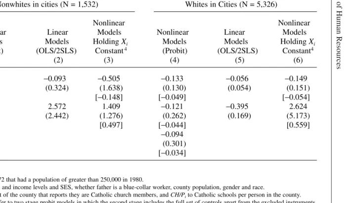
Table 6
Comparison of Linear and Non-Linear Models of College Attendance in NLS-72 (Standard Errors in Parentheses) [Marginal Effects of Nonlinear Models in Brackets]
Sample
Nonwhites in cities (N = 1,532) Whites in Cities (N = 5,326)
Nonlinear Nonlinear
Nonlinear Linear Models Nonlinear Linear Models
Models Models Holding Xi Models Models Holding Xi
(Probit) (OLS/2SLS) Constant4 (Probit) (OLS/2SLS) Constant4
(1) (2) (3) (4) (5) (6)
Single 0.640 0.239 0.253 0.093
equation (OLS/Probit) (0.198) (0.070) (0.062) (0.022)
[0.239] [0.093]
Two equation models Excluded Instruments
%CCHiand CH/Mi 1.471 1.375 5.541 0.048 0.115 0.084
(0.442) (0.583) (2.082) (0.250) (0.158) (0.783)
[0.517] [0.706] [0.018] [0.031]
Ciand %CCHi 0.879 0.054 0.012 −0.090 −0.036 −0.084
(0.523) (0.309) (1.443) (0.121) (0.050) (0.148)
[0.329] [0.004] [−0.033] [−0.031]
Ci, %CCHiand CH/Mi 1.106 0.331 1.302 −0.085 −0.034 −0.069
(0.460) (0.254) (0.706) (0.118) (0.048) (0.125)
[0.409] [0.471] [−0.031] [−0.025]
The Journal of Human Resources
816
Table 6 (continued)
Sample
Nonwhites in cities (N = 1,532) Whites in Cities (N = 5,326)
Nonlinear Nonlinear
Nonlinear Linear Models Nonlinear Linear Models
Models Models Holding Xi Models Models Holding Xi
(Probit) (OLS/2SLS) Constant4 (Probit) (OLS/2SLS) Constant4
(1) (2) (3) (4) (5) (6)
Cionly 0.761 −0.093 −0.505 −0.133 −0.056 −0.149
(0.543) (0.324) (1.638) (0.130) (0.054) (0.151)
[0.285] [−0.148] [−0.049] [−0.054]
Ci×Di 1.333 2.572 1.409 −0.121 −0.395 2.624
(0.516) (2.442) (1.276) (0.262) (0.169) (5.173)
[0.478] [0.497] [−0.044] [0.559]
None 1.224 −0.094
(0.542) (0.301)
[0.446] [−0.034]
Notes:
1. Sample is taken from counties in the NLS-72 that had a population of greater than 250,000 in 1980.
2. All equations control for parents’ education and income levels and SES, whether father is a blue-collar worker, county population, gender and race.
on CHiis smaller in both of these cases than when the more powerful instrument, Ci, is excluded, which seems at odds with the notion that the exclusion restrictions are driving identification. In contrast, 2SLS estimates swing wildly across specifications, with the results being similar to Evans and Schwab (1995) and our own earlier results; we typically find huge effects with standard errors that are sufficiently large that any estimate within the realm of plausibility would not be significantly different from zero at conventional levels. In the most precisely estimated specification involving all three exclusion restrictions, the 2SLS coefficient of 0.331 (0.254) implies a large effect yet is not statistically significant. In the case of the weakest instrument, Ci×Di, the 2SLS coefficient of 2.572 (2.442) is so large that it does not make sense within the linear probability framework, yet it is still not significantly different from zero.
The bivariate probit results for whites are again fairly similar across specifications, although the precision of the estimates now varies with the choice of instrument. In the 2SLS case, both precision and the coefficients themselves are relatively constant except when Ci×Diis used as an exclusion restriction. It appears that in the urban white subsample, the exclusion restrictions are driving a larger share of identification than they are for urban minorities, but that the linear index assumption in conjunction with normality is still playing a large role. Neal (p. 113 in the notes to Table 6) reports that in high school graduation models the standard error of the bivariate probit esti-mate of αrises from 0.476 when only Catholic schools/square mile is excluded from the high school graduation equation to 0.589 when there are no exclusion restrictions, which suggests that functional form is playing a substantial role in identification in the NLSY as well.
One problem in interpreting the 2SLS results in Table 6 and in Evans and Schwab’s and Neal’s data is that both Catholic school and the educational attainment outcomes are binary events, so the imprecision in 2SLS may arise because the linear probabil-ity model provides a poor approximation for these decisions relative to the bivariate probit. With this in mind, in Table 6 we take an alternative approach to examining the extent to which nonlinearities are contributing to identification in the nonlinear mod-els. Columns 3 and 6 present results from two stage probit models in which the first stage models the probability of Catholic high school attendance as
Pr(CHi= 1⎪Xi, Zi) = Φ(Xi′ β +Zi′λ),
where Φ(•) represents the standard normal cdf and Ziis the vector of instruments. The second stage includes the Xivariables as controls, but rather than including an esti-mate of Φ(Xi′ β +Zi′λ) as the key variable as is commonly done, we include separate predicted probabilities holding Xi and Zi constant at their sample means, respec-tively.25The second stage models for college attendance are then
(11) Pr(COLLi=1X Z X Zi, i, i, i)=U9Xilc+a1U(Xlibt+Zlimt)+a2U(Xilbt+Zlimt)C.
Altonji, Elder, and Taber 817
25. In the specifications we use, two stage probit models in which the outcome models include the estimated predicted probability Φ`Xlibt+Zlimtjof Catholic high school attendance yield estimates which are similar