T H E J O U R N A L O F H U M A N R E S O U R C E S • 46 • 3
sued by a state. This main finding is supported with results from individ-ual-level marriage license and Current Population Survey data. The largest effects are found for lower socioeconomic groups.
I. Introduction
Marriage has been shown to be positively related to a number of important outcomes such as higher earnings and productivity (Ahituv and Lerman 2007; Korenman and Neumark 1991), health (Clark and Etile´ 2006; Duncan, Wilk-erson, and England 2006; Frech and Williams 2007; Kenney and McLanahan 2006; Liu and Umberson 2008), better early child cognitive outcomes (Liu and Heiland, Forthcoming), longevity (Felder 2006), and higher self-reported happiness
(Blanch-Kasey Buckles is an assistant professor of economics at the University of Notre Dame. Melanie Guldi is an assistant professor of economics at Mount Holyoke College. Joseph Price is an assistant professor of economics at Brigham Young University, faculty research fellow at the National Bureau of Economic Research, and research fellow at the Institute for the Study of Labor. The authors thank Bill Evans, Hilary Hoynes, Dan Hamermesh, Dan Hungerman, Martha Bailey, two anonymous referees, and semi-nar participants at Columbia University, UC-Merced, University of Connecticut, University of Miami, Baylor University, the Five Colleges Junior Faculty Seminar, and the annual meetings of SOLE and the PAA. Michael Anderson, Amanda Deckelman, Elizabeth Munnich, Jeff Swigert, and Michelle Zagardo provided terrific research assistance and Scott Cunningham shared his data on STD rates. The data used in this article can be obtained beginning six months after publication through three years hence from Kasey Buckles, 436 Flanner Hall, Notre Dame, IN 46556; kbuckles@nd.edu.
[Submitted March 2010; accepted August 2010]
flower and Oswald 2004; Zimmerman and Easterlin 2006).1 As such, researchers
have long been interested in how individuals respond to changes in the cost of marriage, with some emphasis on the effects of public policy on the decision to marry. Policies that have been shown to affect the likelihood of marriage include those that relate to the marriage contract directly (such as minimum-age requirements and divorce laws) and those that affect couples’ economic incentives to marry (such as income taxes or transfer programs).
In this paper, we examine the decision to marry in response to a policy that has not been previously studied—blood test requirements (BTRs) for obtaining a mar-riage license. The BTRs we consider were enacted in the first half of the twentieth century as part of public health campaigns to reduce the spread of communicable diseases and prevent birth defects (Brandt 1985). The laws required couples applying for a marriage license to be screened for certain conditions, commonly rubella or syphilis. However, after penicillin proved to be a cheap and effective treatment for syphilis and vaccines were developed for rubella, these screenings were no longer considered cost-effective. In 1980, 34 states required a blood test in order to receive a marriage license. Nineteen states repealed their laws in the 1980s, and by 2009 only Mississippi still required premarital blood tests.
We investigate the effects of the repeals of the BTRs on the marriage decision. This is an interesting case to consider for several reasons. First, the state law changes we exploit occurred in 34 states over a wide window of time (1980–2008). This provides significant variation and will allow us to separate the effect of the law change and overall shifts in marriage rates. Second, while we will be interested in whether the effects of the policy vary by socioeconomic status or demographic group, the policy itself affected the entire population eligible for marriage in the state. Thus, the population with the potential to be “treated” in our study is much larger than in previous studies of minimum-age requirements or tax and transfer policies, for example. Third, the repeals provide an opportunity to study the effects of a relatively small change in the cost of getting married. The results may be of interest to policymakers considering other policies that directly (required premarital counseling, waiting periods, and license fees) or indirectly (tax and transfer pro-grams) affect the cost of getting married.
There are several ways that a BTR might increase the cost of getting married and induce couples to either obtain their license in another state or decide not to marry at all. First, the act of submitting to a blood test and waiting for results induces a waiting period for a marriage license that might deter spur-of-the-moment marriages. Also, since blood tests are usually paid for by the individual wishing to be married, the BTR increases the dollar cost of marriage. There are also likely to be other nonpecuniary costs associated with going to the doctor and having blood drawn or the potential cost of testing positive for and having to reveal that condition to one’s partner. These costs might be a greater financial burden for certain populations, including those with lower income and lower education levels.
and find that for this group, BTRs deter marriage; the effect is larger for young women and for mothers without a high school degree. The marriage disincentive effect is also larger for women who are geographically further from a state without a BTR. Finally, we consider a sample of young mothers using Current Population Survey data from 1980 to 2008. We again find that if there was a BTR in place, the mother is less likely to be currently married.
In the next section, we discuss the literature on responses to changes in the cost of marriage, and describe in detail the BTRs we study. Section III describes our data sources and methods, and Section IV presents our results. The last section concludes.
II. Background
A. Review of Literature on Changing the Cost of Marriage
Economic theory suggests that changes in the costs or benefits of marriage can affect marriage outcomes such as marriage rates and marriage timing (Alm, Dickert-Conlin, and Whittington 1999; Becker 1981). As the cost (benefit) of marriage rises, the likelihood of marriage falls (rises). Costs or benefits could be pecuniary (such as a marriage tax penalty) or nonpecuniary (security and stability). They could be one-time (such as a marriage license fee) or faced continuously during the marriage (putting the toilet seat down). Much of the theoretical literature focuses on responses to changes in the value of the marriage contract—to bargaining power (Lundberg and Pollack 1996), or to the division of labor (Becker 1981).
Other research has focused on the disincentive effects imbedded in the tax code in which married couples who file jointly are taxed at a higher rate than they would be if they were single and filed separately (Dickert-Conlin and Houser 1998; Alm and Whittington 1999; Eissa and Hoynes 2000). Rasul (2006) finds that unilateral divorce laws decreased marriage rates, because the laws lower the value of marriage by making it easier for one’s partner to leave. Although researchers have often focused on average effects, altering the cost of marriage may have different effects for persons of different socioeconomic status. For example Bitler, Gelbach, and Hoynes (2002) show that welfare reform had opposite effects on marital status for black versus Hispanic women and Loughran (2002) finds that the effects of male wage inequality on women’s propensity to marry vary along both race and education dimensions.
More related to this paper is the small body of work that has considered the effects of public policies that change the cost or availability of the marriage license itself. An example is the literature on the effects of minimum-age requirements for a marriage license. Blank, Charles, and Sallee (2009) find that when states have a higher minimum age for marriage, some marriages are delayed. However, they also find that many young people marry out of their home state to avoid restrictive laws. Dahl (2010) obtains similar results in his work using minimum-age requirements as an instrument for early marriage. These laws are similar to BTRs in that they make the process of obtaining a marriage license more costly for couples who are not eligible to marry in their state but could travel to another (with the cost being effectively infinite for couples too young to marry in any state). We expect that BTRs may have similar effects—deterring marriage for some individuals, and driv-ing others to less restrictive states to obtain their licenses. We explore both possi-bilities below.
B. Blood Test Requirements
Historically, many states have required applicants for a marriage license to obtain a blood test. These tests were for venereal diseases (most commonly syphilis), for genetic disorders (such as sickle-cell anemia), or for rubella. The tests for syphilis were part of a broad public health campaign enacted in the late 1930s by U.S. Surgeon General Thomas Parran.2Parran argued that premarital testing was
neces-sary to inform the potential marriage partner of the risk of contracting a communi-cable disease, and to reduce the risk of birth defects associated with syphilis.3
Ac-cording to Brandt (1985), “by the end of 1938, twenty-six states had enacted provisions prohibiting the marriage of infected individuals” (p. 147). Screenings for genetic disorders and for rubella also were implemented in the interest of minimizing the risk of genetic disease or birth defects in the couple’s offspring.4
2. Our discussion on venereal disease draws primarily from Brandt (1985).
3. Congenital syphilis is strongly linked to blindness and paralysis, and most infants born with the disease died shortly after birth (Brandt 1985).
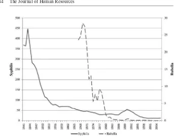
and five cases of congenital rubella were reported nationwide (Reef et al. 2006). Figure 1 shows that incidence rates of both syphilis and rubella had dropped dra-matically by the late 1970s.
These reductions in the prevalence of the diseases, largely due to improvements in medical technology, led to the repeal of the requirements in many states. For example, an article noting the repeal of Massachusetts’ law in 2005 reported that “there are so few syphilis cases now among engaged couples that the test is outdated and an added economic burden . . .. The test also is designed to detect rubella, but people are now vaccinated against that disease” (LeBlanc 2005). While we have found no systematic explanation for why individual states repealed their laws when they did, in the next section we test for possible endogeneity in the timing of the repeals. We find that the repeals are not a function of state levels of marriage rates, rates of syphilis and gonorrhea, or of trends in marriage rates.
It is important to mention that even in the early days of BTRs, there is evidence that couples took steps to avoid the tests (Brandt 1985):
After Connecticut passed its law in 1935, and before the New York Legislature had taken action, weekend marriages in New York counties bordering Con-necticut rose by 55 percent . . . the number of marriages in some states re-portedly declined after premarital exams became legally required. (p. 149). There was also the view that BTRs might discourage marriage altogether: “In New Jersey some state legislators expressed concern that premarital laws that restricted marriage to the healthy could lead to an increase of free love, illegitimacy, and common-law marriages” (p. 149). Thus, our hypothesis that BTRs might decrease marriage licenses issued by a state and possibly deter marriages finds support in the historic record.
Figure 1
Incidence of Syphilis and Rubella in the United States, 1941–2006 (Cases per 100,000)
Source: “Sexually Transmitted Disease Surveillance 2006” (CDC 2007a); “Summary of Notifiable Dis-eases–United States, 1996” (CDC 1997); “Summary of Notifiable DisDis-eases–United States, 2006” (CDC 2007b).
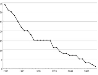
identified 34 states that had a BTR in 1980. Of these 34, 19 states repealed their law in the 1980s, seven repealed in the 1990s, and seven more repealed between 2000 and 2008, leaving only Mississippi with a BTR in 2009.5For our results, a
state-year observation is coded as having a BTR if a requirement was in place for the entire calendar year. Figure 2 shows the number of states with a BTR from 1980 to 2008.6
C. Blood Test Requirements and Marriage
We utilize the within-state variation produced by the repeal of blood test laws to examine the laws’ impact on marriage. The presence of requirements may increase
5. In all of our analysis, we classify the District of Columbia as a state.
Figure 2a
Timing of Blood Test Requirement Repeals, 1980–2008
Figure 2b
the price of obtaining a marriage license in several ways. First, in many cases there is a waiting time of at least a few days between the admission of a blood test and the receipt of the results. Calls to clinics in Washington, D. C. and Mississippi, the two states that still had a test in 2008, found that couples wait three to five days for the results of their tests. Additionally, a couple may need to make an appointment with their physician or local clinic to be tested. Thus, the BTRs introduce a waiting period that could prevent couples who decide to marry on the “spur-of-the-moment” from doing so.7
Further, the presence of a BTR may increase the price of obtaining a marriage license. To comply with a requirement, individuals applying for a marriage license must pay for the doctor’s visit and blood test in most cases, which “can cost couples hundreds of dollars” (Leblanc 2005). Clinics in Washington, D. C. and Mississippi reported per-couple costs of $40 and $26, respectively. In DC, tests from a doctor’s office were reported to cost as much as $200 per couple. Additionally, the Mississippi clinic we called indicated that Medicaid could not be used to cover the cost of the test. There may be other financial costs associated with obtaining the test, including the opportunity cost of the time spent.
Finally, there may be psychological costs associated with a BTR. As Bowman (1977) observes (referring to tests for sickle-cell anemia), “the mandatory testing for carriers of genetically determined diseases at the time of marriage application can result in serious psychological trauma, for the decision has already been made to marry.” Applicants may wish to avoid learning about their disease status, or may want to keep this information from their partners. There also may be nonnegligible disutility from a visit to the doctor, or from the procedure of having blood drawn. Taken together, we believe these costs may have made a BTR a deterrent to obtaining a marriage license in states with the laws, and may have also decreased couples’ likelihood of marrying at all.
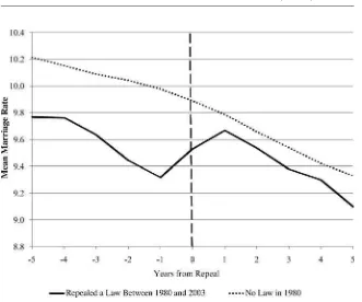
In Figure 3, we provide some graphical evidence of the impact of BTRs on marriage rates. In this figure, we graph the number of marriage licenses issued per 1,000 state residents, before and after the repeal of a BTR. Data are from the CDC’s reports of state marriage rates (described in more detail in the next section). The solid line plots the average of the marriage rates for 27 states that had a requirement in place in 1980, but who repealed their law by 2003. We center the figure at the year the law was repealed in each state and report the marriage rates for the five years before and after the repeal of the law. The dotted line represents a “control” group of 16 states that did not have a blood test law at any time between 1980 and 2003.8For this group, the mean marriage ratetyears from repeal is calculated using
an average of marriage rates in years in which a law was repealed in another state, following Ayers and Levitt (1998).
7. While we have no data on the prevalence of spur-of-the-moment marriages, we do observe the day of the week and type of ceremony in our marriage license data. In 1980, 10.6 percent of marriages were civil ceremonies that took place between Monday and Thursday suggesting that a nontrivial portion of marriages are not of the (presumably planned) weekend-church-wedding-variety. Also, in the 1984 Detroit Area Survey of 459 ever-married women age 18–75, 10.9 percent of the women report that they were never engaged before marrying (White 1990).
Figure 3
Number of States with a Blood Test Requirement, 1980–2008
Source: CDC reports of state marriage rates, 1975–2008. The solid line is the average marriage rate for 27 states that had a blood test requirement in place in 1980 but who repealed the law by 2003. The data for each state are centered at the year the law was repealed. The dotted line corresponds to the 16 states that did not have a blood test requirement in 1980, where the mean marriage rate t years from repeal is calculated using an average of marriage rates in years in which a law was repealed in another state, following Ayers and Levitt (1998). Eight states are not included in the figure for reasons addressed in the data appendix.
III. Data and Methods
We will be using within-state variation in whether states require a blood test for a marriage license to examine the impact of the laws on marriage behavior. The general specification is:
y ⳱Ⳮ*bloodtest Ⳮ␣Ⳮ␦ⳭtimeⳭε
(1) st 0 1 st s t s t st
wherebloodtestst is a dummy variable equal to one if stateshad a blood test for
the entire year in yeart,␣srepresents state fixed-effects,␦tare year dummies,timet
is a quadratic time trend,sgives the state-specific coefficient on the time trend, and
εstis random error. The dependent variable will be a measure of marriage behavior
in statesand period tand will vary with the particular data set and specification. Because errors may be serially correlated within state, we estimate heteroskedastic, robust standard errors that are clustered at the state level.
As with any identification strategy using variation in state laws, one must be concerned with the exogeneity of the laws. Our results will be biased if the presence of a law or timing of a repeal is correlated with unobserved state characteristics. To address this, we include state fixed effects and state-specific quadratic trends in all of our preferred specifications. We also include year dummies in all specifications, to allow for any secular trends in marriage rates. As further checks on the exogeneity of the laws, we test whether the timing of the repeals can be predicted by observed state characteristics, and we consider the effects of adding a placebo law to our main results. We also show that the results are robust to the inclusion of controls for waiting periods and minimum-age laws.9
We use four different panel data sets in our analysis.10First, we use annual state
marriage rates, defined as the number of marriage licenses issued per 1,000 state residents, obtained from the CDC’s Vital Statistics data for 1980–2008. Thus, esti-mating Equation 1 using these marriage rates as the dependent variable will tell us whether the laws had any effect on the number of marriage licenses issued by states. The advantage of this data set is that it is available for the entire time period we are interested in studying, and for all states. States also might be interested in know-ing the effects of the laws on license applications, since marriage license fees are a source of revenue for local and state governments. However, even if we see that the laws decrease marriage licenses, we will not be able to identify decreases in actual marriages using this data set—couples in states with requirements could still be marrying but obtaining their licenses in another state. Furthermore, this data is not available at a more detailed level (for example, subdivided into racial or education categories).
For these reasons, we also use the Marriage and Divorce Detail Files from Vital Statistics, which contain individual-level data from marriage licenses. The data are available from 1981 to 1995, and not all states report their individual license data (see the data appendix). However, the data is ideal for analyzing the impact of a change in blood tests on marriage, as both the state of residence and state of marriage
for children born in and out of marriage.15The model is similar to Equation 1, but
the dependent variable is a binary variable equal to one if the mother is married at the time of birth. We include controls for mother’s race and education, and we divide the sample to test the hypothesis that the BTRs have a greater effect on low-SES women. We also present results using a distance measure of women’s access to a marriage license without a blood test requirement.
Finally, we turn to estimating the effect of the laws on respondents’ reported relationship status in the Current Population Survey from 1980 to 2008. This allows us to examine the effect of BTRs on marriage in a fourth data set, and to also consider the effects of BTRs on women below the poverty line.
IV. Results
A. Effect of Laws on Marriage Licenses Issued
We first estimate the effect of states’ BTRs on the number of marriage licenses issued by the state. The results in Table 1 are based on data from CDC reports of state marriage rates from 1980–2008—the same data that were used to create Figure 3. Each coefficient in the table is the estimate of the effect of the presence of a BTR
11. We also constructed marriage rates by education, but because education is only reported on the marriage license data through 1988, those results are not reported here.
12. Blank, Charles, and Sallee (2009) raise concerns about the accuracy of administrative data, using minimum-age laws for marriage as a case study. They attribute discrepancies in results from administrative and survey data to young couples moving to less-restrictive states or lying on the marriage certificate. We do not expect either of these to be a concern here since there is no legal restriction against marrying outside one’s state of residence.
13. In states where the mothers are not asked the marriage questions directly, marital status is imputed by the NCHS. In 1980, marital status is imputed for seven states; by 2002, only two states (MI and NY) still impute marital status.
14. The age restriction is imposed to avoid the effects of states’ minimum-age laws.
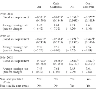
Table 1
Effect of Blood Test Laws on Number of Marriage Licenses Issued by the State, per 1,000 State Residents
State-specific time trends No No Yes Yes
b. Indicates significance at 5 percent. Each coefficient is from a separate regression, where the coefficient is on a dummy indicating whether the state had a blood test requirement in place for the entire year. Standard errors are clustered at the state level and are in parenthesis. Observations are at the state-year level and data are from CDC reports of state marriage rates, defined as the number of marriage licenses issued per 1,000 people. Regressions are weighted by state population. Nevada and Hawaii are dropped from all specifications because of high marriage rates (52.8 and 22.3 respectively in 2006). California is dropped from the second and fourth specifications because of a policy that allowed residents to obtain confidential marriage licenses that did not require a blood test.
on the number of marriage licenses issued per 1,000 state residents (1in Equation
1). We report our results with and without state-specific time trends, and we exclude Hawaii and Nevada from all specifications because of high marriage rates. We ex-clude California from some specifications because of a policy that allowed residents to obtain confidential marriage licenses that did not require a blood test.16We find
on marriage licenses issued is larger post-1995, where the coefficientⳮ0.5821 re-flects a 7.65 percent decrease in marriage licenses issued. We might expect BTRs to have a larger effect in later years for several reasons. The stigma of cohabiting may have lessened in the later period, so that couples are more likely to decide to live together rather than marry in response to a BTR. Decreases in travel costs may have made it easier to travel to another state to obtain a license. As a result, as more states repeal their laws, couples have more options when looking to marry in a state that does not require a test.
As mentioned in the discussion of our empirical strategy, the above results are biased if the presence of a BTR or the timing of a repeal is correlated with unob-served state characteristics. While we cannot test this directly, we perform three exercises that suggest that the repeals can be treated as exogenous. First, we estimate a probit model to test whether observed characteristics impact the probability that a state repeals its BTR, conditional on having not yet repealed.17The estimated
equa-tion is as follows:
repeal ⳱Ⳮ X Ⳮ Z ⳭX *timeⳭ
(2) st 0 1 stⳮ1 2 stⳮ1 3 stⳮ1 t st
whererepealstis equal to one if statesrepealed a BTR in yeartand zero otherwise.
Xstⳮ1is the one-year lagged state marriage rate (defined as above), andXstⳮ1* timet
is the state-specific quadratic marriage rate trend.Zstⳮ1is a vector of one-year lagged
state rates of gonorrhea and syphilis; rates of gonorrhea and syphilis are from the CDC and are defined as the number of reported instances per 100,000 people. The random error isst. The sample begins in 1981 with all states with a BTR in place
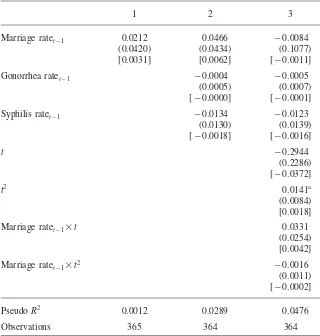
(excluding Hawaii and California), and states exit the sample once a law is repealed. The results are presented in Table 2. We find that these variables are not predictors of the repeal of a law—the coefficients are neither statistically nor practically sig-nificant.
Table 2
Estimated Probit Models for the Repeal of a Blood Test Requirement
1 2 3
Marriage ratetⳮ1 0.0212 0.0466 ⳮ0.0084
(0.0420) (0.0434) (0.1077)
PseudoR2 0.0012 0.0289 0.0476
Observations 365 364 364
a. Indicates significance at the 10 percent level. The dependent variable is equal to one if the state repealed a blood test requirement in that year and zero otherwise. Standard errors are clustered at the state level and are in parenthesis, marginal effects are in brackets. Observations are at the state-year level. The sample is all states with a law in 1981, and states exit the sample once a law is repealed. Marriage rates are from CDC reports, defined as the number of marriage licenses issued per 1,000 people. STD rates are from the CDC, defined as the number of instances per 100,000 people. Hawaii is dropped because of its high marriage rate (22.3 in 2006), and California is dropped because of a policy that allowed residents to obtain confidential marriage licenses that did not require a blood test.
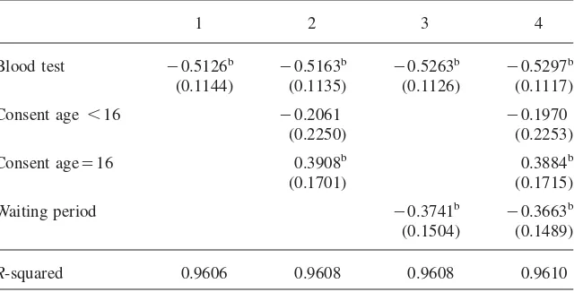
As a second test, we reproduce the main results of Table 1 but add controls for license waiting periods and for minimum-age laws. Information on minimum-age laws was available through 2003, so we restrict our sample to this period. Results are in Table 3. Column 1 shows the effect of BTRs over this period; the coefficient
(0.1504) (0.1489)
R-squared 0.9606 0.9608 0.9608 0.9610
b. Indicates significance at 5 percent. Specification for Column 1 is as in Table 1, Column 4, but with years 2004–2008 omitted due to missing minimum-age law information. The following columns add con-trols for women’s minimum age for marriage with parental consent (age 17–18 is the base case) or for a waiting period. Standard errors are clustered at the state level and are in parenthesis. Observations are at the state-year level and data are from CDC reports of state marriage rates, defined as the number of marriage licenses issued per 1,000 people.
we add indicators for the minimum age for marriage with parental consent for women, where the omitted group is a minimum age of 17 or 18. In Column 3, we add a dummy indicating that the state imposed a waiting period to obtain a marriage license, and Column 4 includes all three policies.
The effect of a BTR is highly robust to the inclusion of these controls, confirming that the repeals were not correlated with other changes in marriage policy. While the effect of a consent age younger than 16 is statistically insignificant, an age of 16 is predicted to increase marriage rates relative to states with a consent age of 17 or 18. Waiting periods have the expected effect—marriage rates are lower in states with a waiting period in place. However, the magnitude of the effect is smaller than the estimated effect of a BTR. This finding is consistent with BTRs imposing a cost similar to a waiting period, plus some additional financial or psychological costs.
We also reproduce the results in Table 1 while adding a placebo law that is repealed two years before each state’s actual repeal. We would expect these placebos to have an effect if states repealed their BTRs in response to changes in marriage rates (so that there is reverse causality in Equation 1). These results are in Appendix Table A1. We find that the placebo law is never statistically significant, and that the effects of the BTRs are virtually unchanged.
Table 4
Effect of Blood Test Laws on Number of Marriages per 1,000 State Residents
All White Black Other
By groom’s state of residence ⳮ0.3014b ⳮ0.3822b ⳮ0.4983 ⳮ0.2343b
(0.0865) (0.0960) (0.3919) (0.1018) By groom’s state, age ⬍30
only
ⳮ0.3947b ⳮ0.6947b ⳮ0.5815 ⳮ0.2122b
(0.1640) (0.1453) (0.3623) (0.1022) By bride’s state of residence ⳮ0.3106b ⳮ0.3735b ⳮ0.5423 ⳮ0.2375b
(0.0938) (0.1025) (0.3900) (0.1110)
State and year fixed effects Yes Yes Yes Yes
State-specific time trends Yes Yes Yes Yes
Mean by groom’s state, all ages
9.10 9.62 7.86 2.42
(Percent change) (ⳮ3.31) (ⳮ3.97) (ⳮ6.34) (ⳮ9.68)
Observations 629 507 507 507
b. Indicates significance at 5 percent. The dependent variable is number of observed marriages for state residents, per 1,000 residents. Standard errors are clustered at the state level and are in parenthesis. Ob-servations are state-year cells, and data are from Vital Statistics Marriage License Records for reporting states, from 1981–95. Regressions are weighted by population. For the regressions done by race, states are also omitted if race is not reported on the license. Maine is omitted in 1995 due to data errors. California is omitted because of a policy that allowed residents to obtain confidential marriage licenses that did not require a blood test. State-specific time trends are quadratic.
marriage license fees are a source of revenue for state and local governments. How-ever, while these results are consistent with the hypothesis that BTRs actually deter marriage, we cannot test this directly with this data. It is possible that the observed decrease in licenses issued is driven by couples who are still getting married, but are just doing so in another state. To study the effect of BTRs on the likelihood of marriage, we turn to results using individual marriage license data.
B. Effect of Laws on Marriages to State Residents
estimate of a 3.3 percent decrease in the marriage rate in response to a BTR is close to that of Alm and Whittington.20
Though the results for blacks are imprecise, the point estimates for racial groups suggest that the BTRs may be more of a deterrent to marriage for blacks than for whites. The coefficientⳮ0.4983 represents a 6.3 percent decrease in marriage rates for blacks, while the effect for whites is a 4.0 percent decrease. When the sample is restricted to marriages where the groom is younger than age 30, the effect of the laws is generally greater in magnitude. These results suggest that BTRs do have more of an impact on lower-SES groups, who might find the economic or other costs of the tests to be a greater deterrent. The results are similar when state marriage rates are constructed using the bride’s state of residence.21
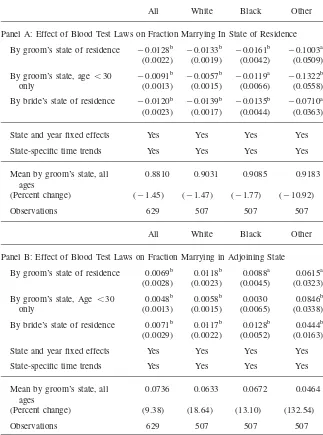
To further explore the issue of couples marrying in other states in response to a BTR, we use data on state of residence and state of marriage to examine the laws’ impact on couples’ likelihood of marrying in their state of residence or in an ad-joining state. These results are reported in Table 5. In Panel A, the dependent variable is constructed by taking the total number of marriages to a state’s residents as the denominator, and the number of those marriages that took place in the state as the numerator. We see that the percent of couples marrying in the groom’s state of
18. The nonreporting states are AZ, AR, NV, NM, ND, OK, TX, and WA.
19. Because individuals from nonreporting states are underrepresented in Table 4, we also have reproduced the result from Table 1 for 1980–95 using only reporting states. The estimated decrease in marriage licenses using this subsample is 4.6 percent.
20. While not directly comparable, the 3.3 percent effect that we observe is smaller than the effect of other policies or factors that influence marriage rates. For example, Angrist (2002) finds that a change in the male-female sex ratio from 1 to 1.25 raised marriage rates by 6 percent. Charles and Luoh (2010) show that a standard deviation increase in the incarceration rate lowers marriage rates by 14 percent. Bitler et al. (2004) find that welfare reform led to a 21 percent decrease in marriage rates.
Table 5
Effect of Blood Test Laws on Where Marriage License is Obtained
All White Black Other
Panel A: Effect of Blood Test Laws on Fraction Marrying In State of Residence
By groom’s state of residence ⳮ0.0128b ⳮ0.0133b ⳮ0.0161b ⳮ0.1003a
(0.0022) (0.0019) (0.0042) (0.0509)
By groom’s state, age ⬍30 only
ⳮ0.0091b ⳮ0.0057b ⳮ0.0119a ⳮ0.1322b
(0.0013) (0.0015) (0.0066) (0.0558)
By bride’s state of residence ⳮ0.0120b ⳮ0.0139b ⳮ0.0135b ⳮ0.0710a
(0.0023) (0.0017) (0.0044) (0.0363)
State and year fixed effects Yes Yes Yes Yes
State-specific time trends Yes Yes Yes Yes
Mean by groom’s state, all
Panel B: Effect of Blood Test Laws on Fraction Marrying in Adjoining State
By groom’s state of residence 0.0069b 0.0118b 0.0088a 0.0615a (0.0028) (0.0023) (0.0045) (0.0323)
By groom’s state, Age ⬍30 only
0.0048b 0.0058b 0.0030 0.0846b (0.0013) (0.0015) (0.0065) (0.0338)
By bride’s state of residence 0.0071b 0.0117b 0.0128b 0.0444b (0.0029) (0.0022) (0.0052) (0.0163)
State and year fixed effects Yes Yes Yes Yes
State-specific time trends Yes Yes Yes Yes
Mean by groom’s state, all ages
0.0736 0.0633 0.0672 0.0464
(Percent change) (9.38) (18.64) (13.10) (132.54)
Observations 629 507 507 507
alternative data sets.
C. Effect of Laws on Marital Status of First-Time Moms
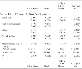
Using the Vital Statistics Natality Detail data, we measure the effect of the laws on the fraction of first-time mothers who are married. Data are collapsed to the state-year level and results are reported in Table 6. First, consider the results in Panel A, for which the specification is again as in Equation 1. For all mothers older than 18, the presence of a BTR in the year of the birth decreases the likelihood of marriage by 0.4 percentage points, or 0.54 percent. For women of lower socioeconomic status, the effect is larger—BTRs decrease the likelihood of marriage by 1.7 percent for black women, by 3.5 percent for women without a high school degree, and by 1.3 percent for women younger than 25. These effects are consistent with those observed using marriage license data, though smaller (perhaps because the marriage decisions of new mothers are less likely to be affected along this margin).23Again, we find
that the laws have a greater effect on low-SES groups.
In Panel B of Table 6, we consider an alternative measure of our policy variable. The variable “distance” is the distance, in hundreds of miles, from the state’s popu-lation centroid to the nearest state without a BTR. For state-years with a blood test requirement for this period, the mean distance in miles is 111, the median is 95, and the range is 4 to 466. Arguably, a BTR in one’s home state should be less of a barrier to marriage if a state without a BTR is nearby. While we have generated results for our other estimates using this variable (see Appendix Tables), we believe the effect of distance may be particularly important for pregnant women, for whom travel may be more difficult.
22. In results not shown here, we replicated the exercise in Table 4 using our distance measure as the policy variable, for states with a BTR in place. The results are statistically insignificant but accord with intuition–among couples who did marry, when the distance to a state without a BTR was greater, they were more likely to marry in-state and less likely to marry in an adjoining state.
Table 6
Effect of Blood Test Laws on Marital Status of First-Time Mothers Ages 19Ⳮ
All Mothers Black
Panel A: Effect of Presence of a Blood Test Requirement
Blood test ⳮ0.004b ⳮ0.006a ⳮ0.017b ⳮ0.008b
(0.002) (0.004) (0.005) (0.002)
High school graduate 0.196b 0.140b 0.128b
(0.007) (0.005) (0.006)
R2 0.8191 0.8150 0.8254 0.9377
All Mothers Black
Panel B: Effect of Distance from State Population Centroid to Nearest State with no Requirement
Distance in miles/100 ⳮ0.003b ⳮ0.003a ⳮ0.007a ⳮ0.005b
(0.001) (0.002) (0.004) (0.002) High school graduate 0.196b 0.140b 0.128b
(0.008) (0.005) (0.006)
R2 0.8209 0.8151 0.8270 0.9398
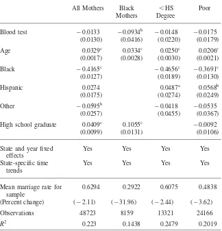
Table 7 shows the results from a linear probability model that controls for race/ ethnicity, age, and education. The results are imprecise, but again suggest that a BTR reduces the likelihood that a young mother is married. The percent effects are quite close to those for the birth certificate results, particularly for women without a high school degree. The results for blacks are an exception; in the CPS we observe a much larger percent effect of a BTR on the probability of marriage. The imprecision of these results leads us to prefer the birth certificate estimates (which have 2,000 times more observations), but we take the CPS results as further evidence of a negative effect of BTRs on marriage.24
V. Conclusion
In this paper, we consider the effect of the repeal of states’ blood test requirements for marriage licenses on marriage. We use a within-group estimator that holds constant state and year effects and exploits the variation in the dates of BTRs across states. We begin with panel data on state marriage rates between 1980 and 2008, and show that blood test requirements decrease marriage licenses issued by a state by 6.1 percent. We also show that the repeals are not correlated with state marriage or STD rates, or in trends in marriage rates, suggesting that we can treat the law repeals as exogenous within our models. We then use individual-level mar-riage license data from 1981 to 1995 to confirm that for this period, about one-third of the decrease in licenses issued by the states was due to couples going out of state for their licenses, while the rest was due to couples deciding not to marry at all. We also use birth certificate data and Current Population Survey data to show that for first-time or young mothers, the likelihood of being married was lower in states with
Table 7
Effects of Blood Test Laws on Marital Status of Mothers Age 19–24
All Mothers Black
Age 0.0329c 0.0334c 0.0250c 0.0206c
(0.0017) (0.0028) (0.0030) (0.0021)
Black ⳮ0.4165c ⳮ0.4656c ⳮ0.3691c
(0.0127) (0.0189) (0.0130)
Hispanic 0.0274 0.0487a 0.0568b
(0.0175) (0.0274) (0.0249)
Other ⳮ0.0595b ⳮ0.0418 ⳮ0.0535
(0.0257) (0.0455) (0.0367)
High school graduate 0.0409c 0.1055c ⳮ0.0092
(0.0099) (0.0131) (0.0106)
R2 0.223 0.1438 0.2479 0.2019
a., b., c. Indicate significance at 10 percent, 5 percent, and 1 percent. Standard errors are clustered at the state level and are in parenthesis. Data are from the 1980–2008 Current Population Survey. California is omitted because of a policy that allowed residents to obtain confidential marriage licenses that did not require a blood test. Includes state and year fixed effects and quadratic state-specific time trends. The blood test variable indicates whether a blood test was in place in that state in the year of the survey
a blood test requirement. Even though all individuals living in states with BTRs faced a higher cost of marriage, we find greater effects for individuals who are black, young, or without a high school degree.
carceration rates (Charles and Luoh 2010). Also, a recent study by Dahl and Moretti (2008) uses child’s gender to show that women pregnant with males are more likely to get married. However, use of these instruments to estimate the causal impacts of marriage can be limited by the somewhat narrowly defined treated population (for example: immigrant populations in the early 20th century, pregnant women).
Our results indicate that blood test requirements provide plausibly exogenous within- and across-state variation in the cost of marriage, and thus might be used to identify the causal effects of marriage. Because the tests were originally enacted in the interest of public health but were repealed after they became obsolete, the effects of the policy change should not directly affect other outcomes such as labor force participation, earnings, or fertility. Further, the BTRs were repealed over a long and recent period in U.S. history and potentially affect the entire population of couples considering marriage in the affected states—though the fact that the laws have the greatest impact for low-SES groups suggests that this strategy might be particularly helpful to researchers studying the effects of marriage for these groups. Along this line, Buckles and Price (2010) use BTRs as an instrument for marriage to study the effect of marriage on infant health for low-SES women.
APPENDIX 1
Data Appendix
1. Information on state blood test requirements was obtained from state statute volumes. A complete list of volumes used is available upon request. We supple-mented our research with searches of newspaper records using Lexis-Nexis. In order to be counted as a repeal, we required that we find two separate articles referring to the repeal. Robles (2010) also uses information on blood test requirements from the state statute volumes in his research which examines the health consequences of repealing blood test laws.
http://www.census.gov/geo/www/cenpop/statecenters.txt. We then used Google Maps to estimate the driving distance from the centroid (given by latitude and longitude) to the nearest state line without a BTR.
3. CDC-Reported Marriage Rates from 1975–2008 were obtained from the website of the Center for Disease Control’s National Center for Health Statistics: http:// www.cdc.gov/nchs/#.
In Figure 3, using this data, eight states are not included: Hawaii and Nevada are omitted because of high marriage rates; California and Oklahoma are omitted for missing data; Massachusetts, the District of Columbia, Mississippi, and Montana are omitted because each still had a law in place as of 2004.
4. Marriage License Data from 1981–95 are from the Vital Statistics Marriage and Divorce Detail Files and are available at http://www.nber.org/data/marrdivo .html. States that do not report marriage license data include Arizona, Arkansas, Nevada, New Mexico, North Dakota, Oklahoma, Texas, and Washington.
Marriage rates, including those by race, are created using population estimates from the United States Census Bureau: http://www.census.gov/popest/states/. These population estimates are also used when weighting the data by state population.
5. Birth Certificate Data (the Natality Detail Files) for 1980–2002 are from the Center for Disease Control’s National Center for Health Statistics. They are available for download at http://www.nber.org/data/vital-statistics-natality-data.html.
6. Current Population Survey data for 1980 to 2008 were obtained from IPUMS: http://www.census.gov/cps/.
7. Gonorrhea and syphilis rates used in Table 1 and Figure 1 were constructed using disease prevalence data from the Center for Disease Control (see references) and state population data from the Census Bureau.
Blood test requirement ⳮ0.6598b ⳮ0.6257b ⳮ0.4253b ⳮ0.4574b
0.2588 0.2909 0.1271 0.1346
Placebo 0.0140 0.0367 0.0016 0.0014
(0.3282) (0.0918) (ⳮ0.0999) (ⳮ0.2364)
Panel C: 1996–2008:
Blood test requirement ⳮ0.8322b ⳮ0.8732b ⳮ0.5673b ⳮ0.5721b
0.1783 0.1726 0.1964 0.1912
Placebo 0.0000 0.0000 0.0058 0.0044
(0.1206) (0.0716) (0.1217) (0.0939)
State and year fixed effects
Yes Yes Yes Yes
State-specific time trends No No Yes Yes
Table A2
Effect of Distance to State with no Blood Test Requirement on Number of Marriages per 1,000 State Residents
All White Black Other
Distance in miles/100 of residence
ⳮ0.1080 ⳮ0.1453b 0.0950 ⳮ0.0292
(0.0657) (0.0716) (0.2039) (0.0402)
State and year fixed effects Yes Yes Yes Yes
State-specific time trends Yes Yes Yes Yes
Mean by groom’s state, all ages
9.09 9.60 7.83 1.89
(Percent change) (ⳮ1.19) (ⳮ1.51) (1.21) (ⳮ1.54)
Observations 599 477 477 477
Hispanic 0.0270 0.0486a 0.0564b
(0.0176) (0.0275) (0.0249)
Other ⳮ0.0505a ⳮ0.0393 ⳮ0.0458
(0.0260) (0.0469) (0.0380)
High school graduate 0.0409c 0.1056c ⳮ0.0093
(0.0099) (0.0131) (0.0107)
State and year fixed effects Yes Yes Yes Yes
State-specific time trends Yes Yes Yes Yes
Mean marriage rate for sample 0.6288 0.2912 0.6070 0.4830 (Percent change) (ⳮ0.00) (ⳮ0.21) (ⳮ0.02) (0.00)
Observations 47,260 8,081 13,069 23,590
R2 0.2240 0.1423 0.2483 0.2024
a., b., c. Indicate significance at 10 percent, 5 percent, and 1 percent. For regression details, see notes to Table 7. Coefficients are for the independent variable “distance,” which is the distance in hundreds of miles from the state population centroid to the nearest state line where a blood test is not required. Hawaii and Alaska are omitted because they do not border other states.
References
Ahituv, Avner, and Robert Lerman. 2007. “How Do Marital Status, Work Effort, and Wage Rates Interact?”Demography44(3):623–47.
Alm, James, Stacy Dickert-Conlin, and Leslie Whittington. 1999. “Policy Watch: The Marriage Penalty.”The Journal of Economic Perspectives13(3):193–204.
Angrist, Joshua. 2002. “How Do Sex Ratios Affect Marriage and Labor Markets? Evidence from America’s Second Generation,”Quarterly Journal of Economics117(3):997–1038. Ayers, Ian and Steven Levitt. 1998. “Measuring Positive Externalities from Unobservable
Victim Precaution: An Empirical Analysis of Lojack.”Quarterly Journal of Economics 113(1):43–77.
Becker, Gary. 1981. “A Treatise on the Family.” Cambridge, Mass.: Harvard University Press.
Bitler, Marianne; Jonah Gelbach, Hilary Hoynes, and Madeline Zavodny. 2004. “The Impact of Welfare Reform on Marriage and Divorce.”Demography41(2):213–36.
Bitler, Marianne, Jonah Gelbach, and Hilary Hoynes. 2002. “The Impact of Welfare Reform on Living Arrangements.”NBER Working Paper No. 8784, February.Cambridge, Mass.: National Bureau of Economic Research.
Blanchflower, David, and Andrew Oswald. 2004. “Well-being over Time in Britain and the U.S.A.”Journal of Public Economics88(7–8):1359–86.
Blank, Rebecca, Kerwin Charles, and James Sallee. 2009. “A Cautionary Tale about the Use of Administrative Data: Evidence from Age of Marriage Laws.”American Economic Journal: Applied Economics1(2):128–49.
Bowman, James. 1977. “Genetic Screening Programs and Public Policy.”Phylon38(2):117– 42.
Brandt, Allan. 1985.No Magic Bullet: A Social History of Venereal Disease in the United States Since 1880. New York: Oxford University Press.
Buckles, Kasey, and Joseph Price. 2010. “Marriage and Infant Health.” Unpublished. Centers for Disease Control and Prevention. 2007. “Sexually Transmitted Disease
Surveillance 2006.” Atlanta, Ga.: U.S. Department of Health and Human Services. Centers for Disease Control and Prevention. 1997. “Summary of Notifiable Diseases—
United States, 1996.”MMWR2007 45(53).
———. 2007. “Summary of Notifiable Diseases—United States, 2006.”MMWR2007; 55(53).
Charles, Kerwin, and Ming Luoh. 2010. “Male Incarceration, the Marriage Market and Female Outcomes.”Review of Economics and Statistics92(3):614–27.
Clark, Andrew, and Fabrice Etile´. 2006. “Don’t Give Up On Me Baby: Spousal Correlation in Smoking Behavior.”Journal of Health Economics25(5):958–78.
Dahl, Gordon. 2010 “Early Teenage Marriage and Future Poverty.”Demography47(3):689– 718.
Dahl, Gordon, and Enrico Moretti. 2008. “The Demand for Sons.”Review of Economic Studies75(4):1085–1120.
Dickert-Conlin, Stacy, and Scott Houser. 1998. “Taxes and Transfers: A New Look at the Marriage Penalty.”National Tax Journal51(2):175–218.
Duncan, Greg, Bessie Wilkerson, and Paula England. 2006. “Cleaning Up Their Act: The Effects of Marriage and Cohabitation on Licit and Illicit Drug Use.”Demography 43(4):691–710.
Eissa, Nada and Hillary Hoynes. 2000. “Explaining the Fall and Rise in the Tax Cost of Marriage: The Effect of Tax Laws and Demographic Trends, 1984–1997.”National Tax Journal53(3):683–711.
Felder, Stefan. 2006. “The Gender Longevity Gap: Explaining the Difference Between Singles and Couples.”Journal of Population Economics19(3):543–57.
Frech, Adrianne, and Kristi Williams. 2007. “Depression and the Psychological Benefits of Entering Marriage.”Journal of Health and Social Behavior48(2):149–63.
Parents’ Marriage on Out-of-Wedlock Children.”Economic Inquiry.
Liu, Hui, and Debra Umberson. 2008. “The Times They Are a Changin’: Marital Status and Health Differentials from 1972 to 2003.”The Journal of Health and Social Behavior, 49(3):239–53.
Lundberg, Shelly, and Robert Pollack. 1996. “Bargaining and Distribution in Marriage.” Journal of Economic Perspectives10(4):139–58.
Moffitt, Robert. 1998. “Welfare, the Family, and Reproductive Behavior: Research Perspectives.”National Academy Press.
Rasul, Imran. 2006. “Divorce Laws and Marriage Markets.”Journal of Law, Economics, and Organization22(1):30–69.
Reef, Susan, Susan Redd, Emily Abernathy, Laura Zimmerman, and Joseph Icenogle. 2006. “The Epidemiological Profile of Rubella and Congenital Rubella Syndrome in the United States, 1998–2004: The Evidence for Absence of Endemic Transmission.”Clinical Infections Diseases43: S126–32.
Ribar, David. 2004. “What Do Social Scientists Know About the Benefits of Marriage? A Review of Quantitative Methodologies.”IZA Discussion Paper No. 998.
Robles, Omar. 2010. “The Health Consequences of Repealing Premarital Blood Testing.” Unpublished.
Robles, Theodore, and Janice Kiecolt-Glaser. 2003. “The Physiology of Marriage: Pathways to Health.”Physiology & Behavior79(3):409–16.
Waite, Linda. 1995. “Does Marriage Matter?”Demography32(4):483–507. Whyte, Martin. 1990. “Detroit Area Study, 1984: The Process of Mate Choice and
Nuptiality in Detroit.” Ann Arbor, Mich.: ICPSR.
Wolfers, Justin. 2006. “Did Unilateral Divorce Laws Raise Divorce Rates? A Reconciliation and New Results.”American Economic Review96(5):1802–20.