in Europe and the United States
New Results
Olivier Bargain
Kristian Orsini
Andreas Peichl
Bargain, Orsini, and PeichlA B S T R A C T
We suggest the fi rst large- scale international comparison of labor supply elasticities for 17 European countries and the United States using a harmonized empirical approach. We fi nd that own- wage elasticities are relatively small and more uniform across countries than previously considered. Nonetheless, such differences do exist, and are found not to arise from different tax- benefi t systems, wage/hour levels, or demographic compositions across countries, suggesting genuine differences in work preferences across countries. Furthermore, three other fi ndings are consistent across countries: The extensive margin dominates the intensive margin; for singles, this leads to larger responses in low- income groups; and income elasticities are extremely small.
Olivier Bargain is affi liated to Aix-Marseille U. (Aix-Marseille School of Economics), CNRS and EHESS. Andreas Peichl is affi liated to ZEW, U. of Mannheim, CESifo, ISER and IZA. Kristian Orsini was affi liated to U. of Leuven at the time the paper was written. The authors are grateful to two anonymous referees, as well as R. Blundell, G. Kalb, D. Hamermesh, A. van Soest and participants to seminars/workshops at UCD, AMSE, IZA, ISER, Leuven, Milan, ZEW. Research was partly conducted during Peichl’s visit to the ECASS and ISER and supported by the Access to Research Infrastructures action (EU IHP Program) and the Deutsche Forschungsgemeinschaft (PE1675). They are indebted to the EUROMOD consortium and to Daniel Feenberg and the NBER for granting them access to TAXSIM. They thank Raj Chetty, Julie Berry Cullen, Hilary Hoynes for providing them with transfer calculators. The ECHP was made available by Eurostat; the Austrian version by Statistik Austria; the PSBH by the Universities of Liège and Antwerp; the Estonian HBS by Statistics Estonia; the IDS by Statistics Finland; the EBF by INSEE; the GSOEP by DIW Berlin; the Greek HBS by the National Statistical Service; the Living in Ireland Survey by the ESRI; the SHIW by the Bank of Italy; the SEP by Statistics Netherlands; the Polish HBS by the University of Warsaw; the IDS by Statistics Sweden; and the FES by the UK ONS through the Data Archive. Material from the FES is Crown Copyright and is used by permission. The usual disclaimer applies. The data used in this article can be obtained beginning January 2015 through December 2017 from the corresponding author: O. Bargain, DEFI, Chateau Lafarge, Route des Milles, 13290 Aix- en- Provence, France. Email: olivier.bargain@univ- amu.fr.
[Submitted July 2012; accepted July 2013]
ISSN 0022- 166X E- ISSN 1548- 8004 © 2014 by the Board of Regents of the University of Wisconsin System
The Journal of Human Resources 724
I. Introduction
The study of labor supply behavior continues to play an important role in policy analysis and economic research. In particular, the size and distribution of work hour and participation elasticities represent key information when evaluating tax- benefi t policy reforms and their effect on tax revenue, employment, and redistribu-tion. Several excellent surveys report evidence on elasticities for different countries and periods.1 However, the literature only reaches a consensus on certain aspects,
establishing that own- wage elasticities are largest for married women and small or sometimes negative for men. In terms of magnitude, large variation in labor- supply elasticities is found in the literature, with little agreement among economists on the elasticity size that should be used in economic policy analyses (Fuchs et al. 1998). For instance, Blundell and MaCurdy (1999) report uncompensated wage elasticities ranging from –0.01 to 2.03 for married women while Evers et al. (2008) indicate huge variation in elasticity estimates. Admittedly, much of the variation across studies is due to different methodological choices, including the type of data used (tax register data or interview- based surveys), selection (for example households with or without children), the period of observation (see Heim 2007), and estimation method. Bar-gain and Peichl (2013) have collected empirical evidence focusing on 15 European countries and the United States. For each demographic group, they observe a large variance in estimates across all available studies, pointing to data year and estima-tion methods as the main sources of variaestima-tion. The authors show that internaestima-tional comparisons based on existing evidence are generally imperfect and incomplete, with insuffi cient common support across studies to conclude about genuine differences in labor- supply responsiveness between countries. The only clear pattern in the literature is that elasticities are larger for women in countries where their participation rate is lower. However, estimates are missing or scarce for several E.U. countries and also some demographic groups, such as childless single individuals. Accordingly, this situ-ation justifi es a serious attempt to estimate labor- supply elasticities for a large number of Western countries in a comparable manner.
Beyond such differences in empirical methods, the following question remains: Do genuine differences that could be explained by different demographic compositions, tax- benefi t systems, labor market conditions, and cultural backgrounds exist between countries? While consistent fi ndings across a large number of countries could make some of the policy recommendations more broadly viable, inversely, contrasted results may explain different policy choices; for instance, different degrees of redistribution between welfare systems. The implicit cost of redistribution between European sys-tems has recently received renewed attention (Immervoll et al. 2007) yet information on actual international differences in labor supply behavior was lacking. Another re-lated question concerns whether participation decisions (the extensive margin) system-atically prevail over responses in terms of work hours (the intensive margin). Indeed, this issue gives rise to the debate about whether welfare programs should be directed
to the workless poor, through traditional demogrant policies, or the working poor, via in- work support (Saez 2001). Large participation responses may subsequently lead to large elasticities in the lower part of the income distribution, which is crucial for welfare analysis. (See Eissa et al. 2008.) Finally, the optimal taxation of couples, and notably the issue of joint versus individual taxation, critically relies on the knowledge of cross- wage elasticities of spouses (Immervoll et al. 2011). At present, empirical evidence on labor- supply responsiveness from an international perspective is virtually absent from the literature.2
The present paper attempts to fi ll this gap, providing the fi rst set of comparable labor supply elasticity estimates for 17 E.U. countries and the United States. For this purpose, we suggest a harmonized approach that nets out possible measurement dif-ferences arising from data, periods, and methods. We benefi t from a unique set of data with comparable variable defi nitions, estimating the same labor supply model for each country. To establish consistent cross- country comparisons, we rely on a structural discrete choice model.3 In this context, the identifi cation is usually obtained by the
nonlinearity of the tax- benefi t code. This present study offers the opportunity to have the complete simulation of all direct tax and transfer instruments for 18 countries at our disposal so that we can fully exploit all nonlinearities and discontinuities in household budget constraints. In addition, we exploit some geographical (for example, across U.S. states) and time variation in tax- benefi t policies for some of the countries, which allows us to estimate elasticities for all demographic groups including childless singles and individuals in couples; this makes the present study very comprehensive compared to existing studies, which typically focus on particular groups.
Our estimations are conducted on 25 representative microdata sets covering 18 countries and two years of data for seven countries. The data sets cover a relatively short time period (1998–2005), which facilitates cross- country comparison. We pro-vide detailed estimates of own- wage elasticities for single individuals and individuals in couples, cross- wage elasticities for couples, and income elasticities for all groups. We analyze the distribution of elasticities across income groups and decompose
2. To our knowledge, only Evers, de Mooij, and van Vuuren (2008) gather evidence for a large set of countries with their meta estimations controlling for different dimensions, including country fi xed effects and methodological differences across studies. However, there may not be enough variation across existing studies, and, moreover, not enough studies per country to isolate genuine international differences from other factors. Furthermore, the special issue of the JHR published in 1990 provided evidence from different coun-tries using variants of the Hausman approach. (See Moffi tt 1990 for an overview.) However, these studies bear methodological differences that prevent their estimates from being directly comparable.
The Journal of Human Resources 726
labor- supply responses between intensive and extensive margins. Using a fl exible random utility model admittedly renders our results immune to the risk of a systematic bias caused by restrictive assumptions on preferences. Nonetheless, we check whether elasticities vary with the form of the utility function, the way we introduce additional
fl exibility (fi xed costs or mass points on certain part- time options), or the hour choice set (from four choices to a much fi ner discretization closer to a continuous model). The complete analysis is based on nine different specifi cations, three demographic groups, and 25 different countries × periods; hence, a total of 675 maximum likelihood (ML) estimations.
Our results show that own- wage elasticities, both compensated and uncompensated, are relatively small and much tighter across countries than suggested by results in the literature. In particular, estimates for married women lie in a narrow range be-tween 0.2 and 0.6, with signifi cantly larger elasticities obtained for countries in which female participation is lower (Greece, Spain, Ireland). Elasticities for married men, expectedly smaller, are even more concentrated while elasticities for single individuals show substantial variation with income levels. Consistent results are also found across countries with important implications for welfare and optimal tax analysis: the ex-tensive margin systematically dominates the inex-tensive margin; for single individuals, this contributes to larger elasticities in low- income groups in most countries; income elasticities are extremely small. The one area where differences remain concerns the cross- wage effects, consistent with substitution in spouses’ household production in Western Europe and complementarity in their leisure in the United States. Using a decomposition analysis, we rule out differences in tax policy, wage/hours levels, and demographics as explanations for cross- country differences in labor supply responses. Accordingly, our results are consistent with Western countries having genuinely dif-ferent individual and social preferences—for example, difdif-ferent preferences for work and childcare institutions.
II. Common Empirical Approach
The principal object of examination in this study is the size of wage and income elasticities, which are standard representations of labor- supply respon-siveness and particularly convenient in terms of conducting international comparisons. While the ideal methodological situation would be to use a generally agreed- upon standard estimation approach, there is no such consensus on this matter. We have opted for the estimation of discrete choice models. This approach is based on the concept of random utility maximization (see van Soest 1995; Hoynes 1996, among others), which requires the explicit parameterization of consumption- leisure prefer-ences, for utility to be evaluated at each discrete alternative. It is not necessary to impose tangency conditions, and in principle the model is very general.4
Labor- supply decisions are reduced to choosing among a discrete set of possibili-ties—for example, inactivity, part- time, and full- time. In this way, both extensive and
intensive margins are directly estimated; the complete effect of the tax- benefi t system is easily accounted for, even in the presence of nonconvexities in budget sets; work costs, which also create nonconvexities; and joint decisions in couples are dealt with in a relatively straightforward manner.
Our methodological choice was guided by two considerations, the fi rst of which involved the need to conduct consistent comparisons across many countries. The only realistic way of doing so was to estimate the same structural, discrete choice model separately for each country, which compels with our attempt to net out all method-ological differences that hinder international comparison. The second key issue is the identifi cation of behavioral parameters, with the main problem that unobserved char-acteristics (for example, being a hard- working person) may infl uence both wages and work preferences to potentially bias estimates obtained from cross- sectional wage variation across individuals. In the traditional approach (for example, in MaCurdy et al. 1990), hours of work are regressed on the aftertax wage and on virtual income. The validity of the instrumental variable estimator hinges on whether the exclusion assumptions of the economic model hold.5 Therefore, a preferred approach consists
of using policy changes to directly identify responses to exogenous variation in net wages. One may rely on a particular tax reform (see Eissa and Hoynes 2004, among others) or long- term variations (Blundell, Duncan, and Meghir 1998; Devereux 2004).6 In our approach, identi
fi cation is mainly provided by nonlinearities, noncon-vexities, and discontinuities in the budget constraint due to the tax- benefi t rules of each country. Closer to the natural experiment method, some exogenous variation also stems from spatial and time variations in these rules, as discussed below.
A. Model and Identifi cation
We opt for a fl exible discrete choice model, as used in well- known contributions for Eu-rope (van Soest 1995; Blundell et al. 2000) or the United States (Hoynes 1996; Keane and Moffi tt 1998). We refer to these studies for more technical details, simply presenting the main aspects of the modeling strategy. In our baseline, we specify consumption- leisure preferences using a quadratic utility function with fi xed costs. Accordingly, the determin-istic utility of a couple i at each discrete choice j = 1, . . . ,J can be written as:
(1) Uij =␣ciCij+␣ccCij2+␣hfiHijf +␣hm iHijm+␣hff(HijF)2+␣hm m(Hijm)2+␣chfCijHijf + ␣chmCijHijm+␣hm hfHijfHijm−jf⋅
1(Hijf >0)−jfm⋅
1(Hijm >0)
with household consumption Cij and spouses’ work hours Hijf and Hijm. The J choices for a couple correspond to all combinations of the spouses’ discrete hours (for singles, the model above is simplifi ed to only one hour term Hij, and J is simply the number of discrete hour choices for this person). Coeffi cients on consumption and work hours are specifi ed as:
5. Estimates are also potentially contaminated by measurement errors (for a discussion of the division bias, see Ziliak and Kniesner 1999).
The Journal of Human Resources 728
(2) ␣ci=␣co+Zic␣c+ui
(3) ␣hfi=␣0hf +Zif␣hf
(4) ␣hmi=␣hm0 +Zim␣hm,
that is they vary linearly with several taste- shifters Zi (including polynomial form of age, presence of children, or dependent elders and region). The term ␣ci also incorpo-rates unobserved heterogeneity, in the form of a normally distributed term ui, for the model to allow random taste variation and unrestricted substitution patterns between alternatives. The normality assumption is mainly made for convenience, and in prin-ciple could be replaced by a more fl exible distribution (for instance, a discrete distri-bution with a fi nite number of mass points, see Hoynes 1996). The fi t of the model is improved by the introduction of fi xed costs of work, estimated as model parameters as in Callan, van Soest, and Walsh (2009) or Blundell et al. (2000). Fixed costs explain that there are very few observations with a small positive number of worked hours. These costs, denoted kj for k = f,m, are nonzero for positive hour choices and depend on observed characteristics (for example, the presence of young children).
As discussed above, this approach allows us to impose very few constraints on the model. In fact, there is nothing to impose in terms of leisure (see van Soest, Das, and Gong 2002). This is especially the case as the utility from leisure is not nonperametri-cally identifi ed from fi xed costs of work. For instance, only very few people work a short week, usually because of these costs—which also could be picked up a fl exible utility function. Furthermore, work may not be a source of disutility, as in textbook models, if staying at home is seen as a depressing activity; namely, fi xed costs of work could be negative for some people. Hence, we do not attempt to interpret them liter-ally—that is as an income defl ator—rather, we express them in utility metric. They may also pick up other, nonmonetary fi xed costs of work, or account for international differences in institutional settings that are not explicitly modeled—for example, dif-ferences in childcare support in the form of subsidies or free childcare at school.7
The only restriction to our model is the imposition of increasing monotonicity in consumption, which seems a minimum consistency requirement for meaningful in-terpretation and policy analysis. Positive marginal utility of consumption is directly imposed as a constraint in the likelihood maximization.8 The potential restrictions due
to the choice of this functional form are examined in Section III.D.
For each labor supply choice j, disposable income (equivalent to consumption in the present static framework) is calculated as a function
7. Note that we refrain from estimating childcare jointly with labor supply. This is not undertaken sys-tematically in the literature, owing to data limitations (notably, the availability and market price of childcare, which can vary locally and with individual circumstances). However, some studies suggest joint estimations; see, for example, Blau and Tekin (2007).
(5) Cij=d(wifHijf,wimHijm,yi,Xi)
of female and male earnings, nonlabor income yi, and household characteristics Xi. The tax- benefi t function d is simulated using calculators that we present in the next section. In the discrete choice approach, disposable income only needs to be assessed at certain points of the budget curve. Male and female wage rates wif and wim for each household i are calculated by dividing earnings by standardized work hours, rather than actual hours, in order to reduce the so- called division bias. We estimate a standard Heckman- corrected wage equation to predict wages. To further reduce the division bias, we predict wages for all observations, rather than only for nonworkers. (Note that we use the inverse Mills ratio in the prediction to account for difference between the two groups.) The two- stage procedure—namely fi rst estimating wage rates and subse-quently using them in the labor supply estimation—is common practice. (See Creedy and Kalb 2005.)9 However, ignoring the wage prediction errors in a nonlinear labor-
supply model would lead to inconsistent estimates of the structural parameters. We take these error terms explicitly into account in the labor- supply estimations, assuming that they are normally distributed and following van Soest (1995).
The stochastic specifi cation of the labor supply model is completed by independent and identically distributed error terms εij for each choice j = 1, . . . ,J. That is, total utility at each alternative is written
(6) Vij=Uij+εij
with Uij defi ned in Expression 1. Error terms are assumed to represent possible ob-servational errors, optimization errors, or transitory situations. Assuming that they follow an extreme value type I (EV- I) distribution, the (conditional) probability for each household i of choosing a given alternative j has an explicit analytical solution: (7) Pij=exp(Uij) / exp(Uik).
k=1
J
∑
The unconditional probability is obtained by integrating out the two disturbance terms— that is, preference unobserved heterogeneity and the wage error term, in the likelihood. In practice, this is achieved by averaging the conditional probability Pij over a large num-ber of draws for these terms so the parameters can be estimated by simulated maximum likelihood. We proceed with simulated ML yet rely on Halton draws of these residuals.10
The Journal of Human Resources 730
status, disability status) or levels of nonlabor income yi, their effective tax schedules are different, that is different actual marginal tax rates or benefi t withdrawal rates.11
In addition, regional variation in tax- benefi t rules generates additional exogenous variation, and can be identifi ed in our data and policy simulations for many countries. For the United States, variation across states in income tax and EITC is a well- known source of variation. (See Eissa and Hoynes 2004; Hoynes 1996.) For E.U. member states, local variation in housing benefi t rules can be identifi ed for some countries in our samples/ simulations (for instance, variations across “départements” in France or municipalities in Finland). In Estonia, Hungary, and Poland, local governments provide different supple-ments to almost all benefi ts, including child benefi ts/allowances and social assistance. For Germany and Italy, regional variation in benefi t rules also exists and is accounted for. Nordic countries operate national and local income taxation, which we account for in the case of Sweden and Finland (with municipal fl at tax rates varying from 16–21 percent in Finland and 29–36 percent in Sweden). In the United Kingdom, the council tax varies between the four main regions. Local taxes on dwelling vary with Belgian regions. Re-gional variations in church tax rates are signifi cant in Finland and Germany while social insurance contributions can vary by region (for example, in Germany).12
Finally, we can avail of two years of data for seven countries. The three- year inter-val between the two corresponding tax- benefi t systems, 1998 and 2001, covers a pe-riod of time where signifi cant tax- benefi t reforms took place. We discuss and explore this additional source of exogenous variation in Section IV.C.
Elasticities. While labor- supply elasticities cannot be derived analytically in the present nonlinear model, they can be calculated by numerical simulations using the estimated model. For wage (income) elasticities, we simply predict the change in aver-age work hours and participation rates following a marginal uniform increase in waver-age rates (nonlabor income). We have checked that results are similar when wage elastici-ties are calculated by simulating either a 1 percent or a 10 percent increase in gross wages (unearned incomes). For income elasticities, we give a marginal amount of capital income to households with zero capital income in order to include them in the calculation. For couples, cross- wage elasticities are obtained by simulating changes in female (male) hours when male (female) wage rates are increased. Standard errors are obtained by repeated random draws of the model parameters from their estimated distributions and recalculating elasticities for each draw.
B. Data, Selection, and Tax- Benefi t Simulations
We focus on the United States, the E.U. 15 member states (except Luxembourg), and three new member states (NMS), namely Estonia, Hungary, and Poland.13 For each
11. Arguably, some of these characteristics are included in Zi and also affect preferences so the model is only parametrically identifi ed. In practice, tax-benefi t rules depend on characteristics Xi, which are much more detailed than usual taste-shifters Zi. For instance, benefi t rules depend on the detailed age of all children in the household, on more detailed geographical information, etc.
12. However, detailed information on regions is missing for Spain, Denmark, Austria, and Portugal (coun-tries for which we use the ECHP data), as well as the Netherlands.
country, we draw information about incomes and demographics that can be used for detailed tax- benefi t simulations and labor- supply estimations from standard house-hold surveys (data sources are specifi ed in Appendix 1). For the EU- 15, the data sets have been assembled within the framework of the EUROMOD project (see Sutherland 2007) and combined with tax- benefi t simulations for either 1998, 2001, or both. When available we use both data years for a country. For the NMS, data were collected only for 2005, and policies simulated for that year, in a more recent development of the EUROMOD project.14 For the United States, we use the 2006 Current Population
Survey (IPUMS- CPS), which contains information for 2005. Data sets have been har-monized within the EUROMOD project, in the sense that similar income concepts are used together with comparable variable defi nitions (for example for education). We explain this in more detail in Appendix 1 and, for the wage estimation, in Appendix 2. For each country, we extract three samples for the purpose of labor supply estima-tions: couples, single men, and women (which include single mothers). We only retain households where adults are aged between 18 and 59, available for the labor market (not disabled, retired, or in education), and we also exclude self- employed, farmers, and “extreme” situations, including very large families and those who report implau-sibly high levels of working hours.
Tax- benefi t Simulations. For each discrete choice j and each household i, dis-posable income Cij is obtained by aggregating all sources of household income and calculating benefi ts received and taxes and social contributions paid. We cover all direct taxes (labor and capital income taxes), social security contributions, family, and social transfers. These tax- benefi t calculations, represented by function d() in Expression 5, are performed using tax- benefi t simulators together with information on income and sociodemographics Xi (for instance, the children composition affect-ing benefi t payments), as previously indicated. For Europe, we use EUROMOD, a calculator designed to simulate the redistributive systems of all the EU- 15 countries and of some of the NMS, which includes simulation of all direct taxes, payroll tax (social security contributions), social, and family benefi ts. An introduction to EU-ROMOD, a descriptive analysis of taxes and transfers in the European Union and robustness checks is provided by Sutherland (2007). EUROMOD has been used in several empirical studies, notably in the comparison of European welfare regimes by Immervoll et al. (2007, 2011). For the United States, calculations of direct taxes, contributions, and tax credits (EITC) are conducted using TAXSIM (version v9), the NBER calculator presented in Feenberg and Coutts (1993), augmented by simulations of social transfers (TANF, Food Stamp). Tax- benefi t simulations for the United States are used in combination with CPS data in several applications (for example, Eissa, Kleven, and Kreiner 2008).15 We assume full bene
fi t takeup and tax compliance. More refi ned estimations accounting for the stigma of welfare program participation—as, for example, in Keane and Moffi tt (1998) or Blundell et al. (2000)—would require precise data information on the actual receipt of benefi ts, which is not always
avail-14. We make use of policy/data years available in EUROMOD at the time of writing (1998, 2001, or 2005, as indicated above), while its future developments should enable extending our results to more the recent period and more countries.
The Journal of Human Resources 732
able or reliable in interview- based surveys. Chan (2013) has recently suggested an extension of Keane and Moffi tt (1998) to a dynamic discrete- choice model of la-bor supply with welfare participation as well as time limits and work requirements. While these features are important in the U.S. context, they are less so for European countries.
Statistics. Descriptive statistics of the selected samples are presented in Appen-dix 1. For married women, mean worked hours show considerable variation across countries, which is essentially due to lower labor market participation in southern countries (with the noticeable exception of Portugal), Ireland and, to a lesser extent, Austria and Poland. While the correlation between mean hours and participation rates is 0.92, there is some variation in work hours among participants, with shorter work duration in Austria, Germany, Ireland, the Netherlands, and the United Kingdom. The participation of single women is lower in Ireland and the United Kingdom due to the larger frequency of single mothers. (The average number of children among single women is highest in these two countries and Poland.) There is much less variation for men, with the main notable fact being a lower participation rate for single compared to married men. Moreover, the variation in wage rates and demographic composition across countries is also noteworthy. Especially for married women, participation rates are correlated with wage rates (corr = 0.36) and the number of children (–0.61). At-tached to these patterns, there may be interesting differences across countries in the responsiveness of labor supply to wages and income, and we turn to this central issue in the next sections. In Appendix 1, we take a closer look at the distribution of actual worked hours. For men, this shows the strong concentration of work hours around full time (35–44 hours per week) and nonparticipation. There is more variation for women, particularly with the availability of part- time work in some countries: A peak at 15–24 hours can be seen in Belgium or 25–34 hours in France, where some fi rms offer a 3/4 of a full- time contract, while the Netherlands shows high concentration in these two segments. The United States is characterized by a particularly concentrated distribution, around full- time and inactivity, and a relatively high rate of overtime. To accommodate the particular hours distribution of each country while maintain-ing a comparable framework, we suggest a baseline estimation usmaintain-ing a seven- point discretization—that is, J = 7 for singles and J = 7 × 7 for couples, with choices from 0 to 60 hours/week (steps of ten hours). Below, we check the sensitivity of our results to alternative choice sets.
III. Results
Before presenting and discussing a large set of results regarding elas-ticities, we comment on the model estimation and how it fi ts the data.
A. Estimates and Goodness- of- Fit
can say that parameter estimates are broadly in line with usual fi ndings. For instance, as expected, the presence of children signifi cantly decreases the propensity to work for women, both in couples and single mothers, in most countries. Taste shifters related to age are often signifi cant for women in couples yet not systematically for other demographic groups. The constant of the cost of work is signifi cantly positive for all groups while the presence of young children most often has a signifi cantly positive impact on the work cost of women. For single men and women, higher education leads to lower costs, which can be interpreted as demand- side constraints in the form of lower search costs. (See van Soest, Das, and Gong 2002.) We cannot truly directly compare preferences across countries, given the large number of model parameters. While a simpler model would allow us to do so—for instance, a LES specifi cation—it would certainly be too restrictive. Hence, we directly focus on the comparison of labor supply elasticities in the next subsection.
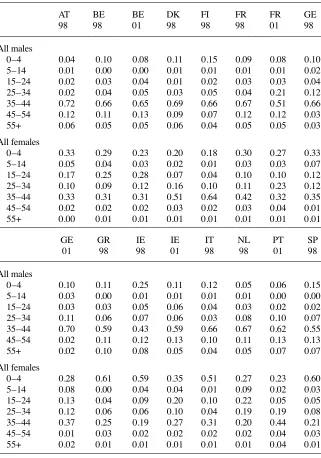
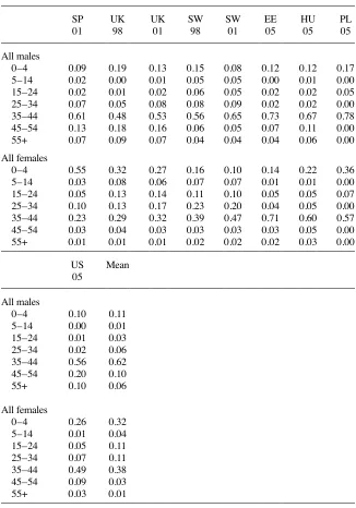
Log- likelihood and pseudo coeffi cient of determination (R2), reported with the es-timates in Appendix 3, convey that the fi t is reasonably good: 0.31 on average for couples (0.28 for singles), from 0.23 for the United Kingdom to 0.45 for Poland (from 0.14 to 0.40 for singles). For couples, Table 1 shows that mean predicted hours compare well with those observed, with the discrepancy less than 1 percent in most cases. There are some exceptions, with larger discrepancies for women in Portugal, Greece, and Spain. For the two latter countries, we report the distribution of observed and predicted frequencies for each choice underneath Table 1. We use a four- choices model for the ease of reading, reporting the 16 combinations (Hr, Hm) for couples. We can see that the option (40, 40) is slightly underestimated, while option (0, 40) is overpredicted. However, the overall distributions of observed and predicted hours even compare relatively well for these countries. For all countries, we have checked that satisfying comparisons at the mean do not hide wrong hour distributions. As an illustration of this, we report two additional graphs in cases where mean hours are correctly predicted (France and the Netherlands), confi rming that the underlying dis-tributions of predicted and observed choices are also well in line. Indeed, these same conclusions are obtained for the model with J = 7 choices. For single individuals, mean predicted and observed hours compare well for many countries, as shown in Table 2. However, the fi t is not as good as for couples, which is a typical result in the literature (Blundell and MaCurdy 1999).16 The discrepancy is less than 5 percent
in almost all cases. For three cases with the largest discrepancies (Belgian women 1998, Irish men 1998, and Portuguese women 2001), we present the hour distributions underneath Table 2 (baseline situation with seven choices). Differences are generally due to bad predictions in terms of participation, as is the case for Irish single men (Por-tuguese single women), where nonparticipation is over(under)predicted. It is also due to the model not being able to reproduce the hours distribution for the workers well. This is the case for Belgian women, for whom participation rates are well predicted yet part- time options are overpredicted at the expense of full- time. This is also the case when the overall fi t is good, such as in the case of French men 2001 reported in our
The Journal of Human Resources
734
Table 1
Predicted and Observed Mean Hours: Couples
AT BE BE DK FI FR FR GE GE GR IE IE IT
98 98 01 98 98 98 01 98 01 98 98 01 98
Female Observed 16.8 24.0 24.3 29.5 32.0 23.1 23.2 19.6 20.7 13.3 11.0 17.5 15.5
Predicted 17.3 24.2 24.2 29.1 31.3 22.9 23.2 19.6 21.1 12.6 10.7 17.2 15.4
Gap (percent) 2.6 0.7 –0.1 –1.1 –2.3 –0.8 –0.2 –0.1 2.0 –5.1 –2.7 –1.5 –1.0
Male Observed 40.3 39.0 39.4 38.3 37.5 38.2 37.0 35.3 35.6 37.9 31.9 36.7 36.0
Predicted 40.5 38.1 38.5 38.4 37.0 38.1 37.0 35.6 35.6 37.6 31.3 36.2 36.5
Gap (percent) 0.4 –2.3 –2.5 0.2 –1.3 –0.1 –0.2 0.9 –0.1 –0.8 –1.9 –1.4 1.4
NL PT SP SP UK UK SW SW EE HU PL US
01 01 98 01 98 01 98 01 05 05 05 05
Female Observed 18.2 26.4 12.0 14.7 20.8 22.1 28.4 30.7 33.2 28.6 23.4 27.0
Predicted 18.3 28.2 12.3 13.5 21.2 22.7 28.7 30.8 33.7 28.6 23.5 26.6
Gap (percent) 0.4 7.0 2.8 –7.8 1.8 3.1 1.0 0.3 1.3 0.2 0.3 –1.3
Male Observed 39.2 39.6 36.8 38.9 37.1 37.1 35.8 37.1 35.9 37.4 33.3 41.1
Predicted 39.1 39.8 36.3 38.2 37.6 37.9 36.2 37.2 36.4 37.3 33.3 40.9
The Journal of Human Resources
736
Table 2
Predicted and Observed Mean Hours: Singles
AT BE BE DK FI FR FR GE GE GR IE IE IT
98 98 01 98 98 98 01 98 01 98 98 01 98
Female Observed 28.8 25.3 27.4 28.6 31.2 29.7 28.1 25.9 26.8 21.6 17.4 22.5 27.3
Predicted 30.2 23.2 26.5 28.6 30.4 29.5 28.2 25.1 25.9 20.4 17.7 23.9 27.1
Gap (percent) 4.6 –8.4 –3.4 0.2 –2.7 –0.4 0.3 –2.9 –3.2 –5.9 1.4 6.0 –0.4
Male Observed 36.8 35.1 34.6 32.9 30.4 33.5 32.2 31.9 32.6 31.6 24.7 27.2 28.8
Predicted 37.2 34.1 34.0 32.2 28.9 33.3 32.1 31.6 31.4 30.6 22.9 24.9 28.7
Gap (percent) 1.2 –2.9 –1.7 –2.0 –5.0 –0.5 –0.3 –0.7 –3.9 –3.0 –7.5 –8.4 –0.3
NL PT SP SP UK UK SW SW EE HU PL US
01 01 98 01 98 01 98 01 05 05 05 05
Female Observed 25.1 28.2 26.1 27.4 20.0 22.2 25.8 29.8 33.4 33.4 26.2 32.7
Predicted 25.9 29.8 25.6 28.4 20.3 22.6 25.9 29.5 33.2 33.2 26.3 32.7
Gap (percent) 3.2 5.7 –2.0 3.3 1.5 1.9 0.3 –1.0 –0.5 –0.5 0.4 –0.2
Male Observed 35.1 32.1 27.5 32.8 28.9 32.1 26.6 31.9 30.4 32.8 23.0 36.2
Predicted 34.3 33.4 27.0 32.8 28.7 32.2 26.5 30.6 30.6 32.5 22.9 35.9
Bar
gain, Orsini, and Peichl
737
0.00 0.10 0.20 0.30 0.40 0.50
0 10 20 30 40 50 60
weekly hours 0.00
0.10 0.20 0.30 0.40 0.50
0 10 20 30 40 50 60
weekly hours
France 2001 (men)
0.00 0.10 0.20 0.30 0.40 0.50 0.60
0 10 20 30 40 50 60
weekly hours
observed
predicted
Portugal 2001 (women)
0.00 0.10 0.20 0.30 0.40 0.50 0.60
0 10 20 30 40 50 60
weekly hours
observed
The Journal of Human Resources 738
illustration.17 The overall conclusion is that the model performs relatively well, which
provides reassurance regarding the reliability of our elasticity measures.
B. The Size of Own- Wage Elasticities
Our main results on labor supply elasticities are illustrated in the graphs below, and are also reported in the Appendix 4 tables, which contain detailed own- wage hour elasticities, compensated and uncompensated, overall, and for quintiles of disposable income.18 We start with own- wage elasticities, as reported in Figure 1.19
Results for Married Individuals. We fi rst focus on married women, the group mostly studied in the literature.20 Total hour elasticities are to be found in a very narrow range
0.2–0.4 for several countries (Austria, Belgium, Denmark, Germany, Italy, and the Netherlands), while they are slightly smaller, around 0.1–0.2, yet signifi cantly differ-ent from zero, in France, Finland, Portugal, Sweden, the NMS, the United Kingdom, and the United States. Furthermore, they are signifi cantly larger, between 0.4 and 0.6, in Ireland (1998), Greece, and Spain. Accordingly, our results show that elasticities are relatively modest and hold in a narrow interval, comparable once data sets, selec-tion, and empirical strategies are used.21 However, estimates are suf
fi ciently precise so that differences between the three aforementioned groups of countries are statistically signifi cant. Over all countries and periods, the mean hour elasticity is 0.27 with a standard deviation of 0.16. The simple intuition that elasticities are larger when female participation is lower is broadly confi rmed by the data; that is, the cross- country cor-relation between mean wage hour (participation) elasticities and mean worked hours (participation rates) is around –0.81 (–0.84). In Tables A8–A9, we show that elastici-ties are only slightly larger for women with children. They are signifi cantly larger in a few countries and notably in the high- elasticity group (Greece, Spain, and Ireland
17. In order to compare the within-sample fi t with out-of-sample predictions, we have also estimated the baseline model on a random half of the sample for each country, subsequently using it to predict hours for the other half. Fit measures on the holdout sample show similar results as those discussed in the text, thus conveying that the fl exible model used does not overfi t the data in a way that would reduce external validity. 18. For the sake of a clear exposition, the graphs focus on the most recent year when two years are available. Appendix tables report detailed estimates for both years, based on separate estimations for each year. As we show below, preferences are relatively stable over the three-year interval considered in this case.
19. We focus on uncompensated elasticities. As reported in Appendix Tables A8–A11, compensated own wage elasticities are only slightly larger than uncompensated ones in most cases, owing to very small and negative income elasticities, as discussed below. They are slightly smaller in rare cases where income elastici-ties are positive, such as single women in Denmark.
20. Bargain and Peichl (2013) show that this statement is particularly true for Europe. Among all studies surveyed, they report 40 estimates for married women, 24 for married men, and 24 for single individuals (including single mothers). For the United States, they report 11 estimates for married women, nine for mar-ried men and six for single individuals (including single mothers).
Bargain, Orsini, and Peichl
0 Own-wage elasticity.2 .4 .6 .8
UK01
0 Own-wage elasticity.2 .4 .6 .8
The Journal of Human Resources 740
1998).22 For married men, results are even more compressed, with own- wage
elastici-ties usually ranging between around 0.05 and 0.15 (see Figure 1). Over all countries/ periods, the mean hour elasticity is 0.10, with a standard deviation of 0.05. Estimates are precise enough to fi nd statistical differences across some countries yet are less pronounced than for women. The correlation between elasticities and worked hours (participation) is around –0.41 (–0.64). Compared to some of the older literature, we
fi nd total hour elasticities that are signifi cantly larger than zero. However, as discussed below, pure intensive margin elasticities are very close to zero.
Results for Single Individuals. While there are numerous studies on the labor supply of single mothers in the United Kingdom and the United States, by contrast, and de-spite the large increase in the number of childless single individuals over the last few decades, the labor- supply behavior of single women and men has received relatively little attention. The main reason is probably that most of the policy reforms used to estimate labor supply responses in the United States and the United Kingdom con-cerned families with children. In this way, the present study adds valuable information to the literature by providing new estimates for all three groups and many countries. As seen in Figure 1, elasticities for single men show a little more variation than for married men, usually in a range between 0 and 0.4. They are signifi cantly different from zero in most cases, with some exceptions. Overall, estimates are slightly larger than for married men, which is in line with lower participation rates and attachment to the labor market among young single individuals. This is particularly the case in Spain and Ireland, where estimates are signifi cantly larger than in other countries. The number of single men with children is marginal and we do not need to discuss it. We observe some variation among single women (mean estimates for the pooled child-less women and single mothers), usually between 0.1 and 0.5 with larger elasticities for some countries (around 0.6–0.7 in Belgium and Italy). Single mothers tend to have larger elasticities than childless women yet differences are usually not signifi cant (with notable exceptions of Greece and Ireland).23 The correlation between elasticities
and worked hours (participation) among single individuals is usually smaller than for couples: –0.50 (–0.50) for women and –0.32 for men (–0.46).
C. International Comparisons
We have established that international differences in the magnitude of wage elastici-ties are modest provided comparable data sets, selection, and a common empirical
22. Appendix Table A1 shows that the number of couples with children is large in Ireland yet close to aver-age in Greece and Spain. Hence, higher elasticities among married women in these countries do not seem to be driven by a higher proportion of families with children. This is confi rmed by the decomposition analysis in the last section.
approach are used. This is an interesting result, given the substantial differences across countries in terms of labor market conditions, institutions, and preferences/culture. Nonetheless, we have found signifi cant differences between broad groups of countries, as discussed above, which we investigate more thoroughly in Section IV. We now focus on interesting regularities and salient differences between countries.
Extensive versus Intensive Margins. In Figure 2, we decompose total hour elastici-ties (that is, changes in total work hours due to a marginal wage increase) into hour changes among workers (intensive margin) and hour changes due to participation re-sponses (extensive margin), and clearly see that most of the response is driven by the extensive margin. This result is important for tax and welfare analyses, as motivated in the introduction. The literature has documented this for a few countries. (See Heckman 1993 for the United States; Bargain and Peichl 2013 for many countries).24 However,
our results show that this pattern holds almost systematically across many Western countries and for all demographic groups. Even in the rare situations where the inten-sive margin is nonzero, the exteninten-sive margin is larger (for example, for Dutch married women). For singles, largest participation responses come from low- income groups, as discussed in further detail below.
The intensive elasticities are extremely small for all countries and all demographic groups—for example, lower than 0.08 for married women in all countries (except the Netherlands). Intensive margin elasticities are sometimes negative for men in couples (for example in the United Kingdom), single men (for example, Belgium, Portugal, and Ireland 1998), and single women (Denmark). Small responses at the intensive margin are mainly due to the few possibilities of working part- time in most coun-tries. Among exceptions where responses are signifi cant, the extreme case is married women in the Netherlands, with an intensive margin representing almost half of the re-sponse. We conjecture that this is due to the outstanding role of part- time work in this country and the possibility of adjusting labor supply along this margin. (On average, around 25 percent of prime- age working women work part- time in the OECD, around 50 percent do in the Netherlands: Compare Table A2 and the discussion in the data section.) Supply- side interpretations of hour restrictions—for example, in terms of job search—are discussed in the robustness checks below and the concluding section. Distribution of Own- wage Elasticities by Income Groups. In the tables of Appendix 4, we provide the distribution of own- wage elasticities of total hours by quintiles of the income distribution (with quintiles defi ned for couples and singles separately). This information is represented graphically in Figure 3, with a box- plot showing the cross- country dispersion for each quintile. In Figure 4, we show the detailed distribu-tion of elasticities across quintiles, separately for each country. The fi rst striking result is that there is much more variation than when only considering mean elasticities. For all groups except married men, elasticities for some income quintiles can go up to one. More precisely, for single individuals, the distribution of elasticities across income groups shows a clearly decreasing pattern, with largest elasticities for lower quintiles. The fact that elasticities may be very heterogeneous across different earning
The Journal of Human Resources 742
0 Own-wage elasticity.2 .4 .6 .8
UK01
0 Own-wage elasticity.2 .4 .6 .8
Bar
gain, Orsini, and Peichl
743
0 .2 .4 .6 .8
Own-wage elasticity
0 .2 .4 .6 .8
Own-wage elasticity
0 .2 .4 .6 .8 1
Own-wage elasticity
Single men
0 .2 .4 .6 .8 1
Own-wage elasticity
Single women
Note: The bottom (middle) [top] of the box are the 25th (50th) [75th] percentile. The ends of the whiskers represent 1.5 times the interquartile range.
Q1
Q2
Q3
Q4
Q5
Figure 3
The Journal of Human Resources 744
0 .2 .4 .6 .8
AT
9
8
BE01 DK98 EE05 FI98 FR01 GE01 GR98 HU05 IE01 IT98 NL01 PL05 PT01 SP01 SW01 UK01 US05 Mean
1 2 3 4 5 1 2 3 4 5 1 2 3 4 5 1 2 3 4 5 1 2 3 4 5 1 2 3 4 5 1 2 3 4 5 1 2 3 4 5 1 2 3 4 5 1 2 3 4 5 1 2 3 4 5 1 2 3 4 5 1 2 3 4 5 1 2 3 4 5 1 2 3 4 5 1 2 3 4 5 1 2 3 4 5 1 2 3 4 5 1 2 3 4 5 Married women
0 .05 .1 .15 .2
AT
9
8
BE01 DK98 EE05 FI98 FR01 GE01 GR98 HU05 IE01 IT98 NL01 PL05 PT01 SP01 SW01 UK01 US05 Mean
1 2 3 4 5 1 2 3 4 5 1 2 3 4 5 1 2 3 4 5 1 2 3 4 5 1 2 3 4 5 1 2 3 4 5 1 2 3 4 5 1 2 3 4 5 1 2 3 4 5 1 2 3 4 5 1 2 3 4 5 1 2 3 4 5 1 2 3 4 5 1 2 3 4 5 1 2 3 4 5 1 2 3 4 5 1 2 3 4 5 1 2 3 4 5 Married men
0 .5 1 1.5
AT
9
8
BE01 DK98 EE05 FI98 FR01 GE01 GR98 HU05 IE01 IT98 NL01 PT01 SP01 SW01 UK01 US05 Mean
1 2 3 4 5 1 2 3 4 5 1 2 3 4 5 1 2 3 4 5 1 2 3 4 5 1 2 3 4 5 1 2 3 4 5 1 2 3 4 5 1 2 3 4 5 1 2 3 4 5 1 2 3 4 5 1 2 3 4 5 1 2 3 4 5 1 2 3 4 5 1 2 3 4 5 1 2 3 4 5 1 2 3 4 5 1 2 3 4 5 Single men
0 .5 1 1.5
AT
9
8
BE01 DK98 EE05 FI98 FR01 GE01 GR98 HU05 IE01 IT98 NL01 PL05 PT01 SP01 SW01 UK01 US05 Mean
1 2 3 4 5 1 2 3 4 5 1 2 3 4 5 1 2 3 4 5 1 2 3 4 5 1 2 3 4 5 1 2 3 4 5 1 2 3 4 5 1 2 3 4 5 1 2 3 4 5 1 2 3 4 5 1 2 3 4 5 1 2 3 4 5 1 2 3 4 5 1 2 3 4 5 1 2 3 4 5 1 2 3 4 5 1 2 3 4 5 1 2 3 4 5 Single women
total (hours) extensive (hours)
Figure 4
groups—and that participation elasticities can be signifi cantly larger at the bottom of the distribution—is crucial for welfare analysis. (See Eissa, Kleven, and Kreiner 2008; Saez 2001.) However, very few studies report this kind of information.25 Our results
generalize it, and show that participation elasticities indeed drive the large responses in lower quintiles for single individuals.
Results for married women do not show such a pattern, in fact pointing to larger elasticities at the top, while Eissa (1995) fi nds similar results for the United States. This is consistent with the added worker theory (see Blundell, Pistaferri, and Ekstein 2012)—namely that women in poor households must complete family income while the labor supply of those in wealthier families is sensitive to fi nancial incen-tives. For married men, our results show a fl at or decreasing pattern, closer to that of singles, although there are some exceptions (that is an increasing pattern in France, Italy, Spain, and the United Kingdom). Results are usually not driven by a decreas-ing intensive margin, but, again, rather by the participation margin. In fact, for some countries like the United States, elasticities decrease with income along the extensive margin while the intensive margin (the difference between total and extensive effects in Figure 4) seems to increase with income. This is in line with the elasticity of taxable income literature, which reports more responses at the top (admittedly due to margins not accounted for here, yet also to more adjustment possibilities for top earners). Other countries (for example, the United Kingdom) show intensive elasticities becoming negative for higher incomes, more in line with backward- bending labor supply curves.
Cross- wage Elasticities. Perhaps the most interesting difference across countries is the measure of cross- wage elasticities within couples, with estimates of uncompen-sated elasticities plotted with confi dence intervals in the lefthand side graph of Figure 5 and reported in the tables of Appendix 4. While these are usually negative and smaller in absolute value than own- wage elasticities, they are nonetheless sizeable for women in some countries, including Austria, Denmark, Germany, and Ireland, which is not an unusual result. (See, for example, Callan, van Soest, and Walsh 2009.) Cross- wage elasticities are much smaller (in absolute terms) for men, between –0.05 and 0 in most countries. Income effects being small, compensated cross- wage elasticities are close to uncompensated ones. We plot compensated elasticities for both men and women on the righthand side graph of Figure 5, in order to easily check the complementarity or substitution between spouses’ working hours. With suffi cient complementarity, an increase in one spouse’s wage must increase both spouses’ working hours—that is, cross- wage elasticities are positive. Interestingly, this situation seems to characterize the United States. (Elasticities are small but signifi cant.) It sounds reasonable that spouses enjoy spending time together, and all the more so as free time is relatively more scarce than in Europe and more likely to coincide with pure leisure. An alterna-tive explanation could be higher assortaalterna-tive mating on productivity levels (compared to Europe). However, recent evidence in an intertemporal framework by Blundell, Pistaferri, and Saporta- Ekstein (2012) tends to support the former explanation. By contrast, our results point to substitutability between male and female working hours
The Journal of Human Resources
EE05 UK01 PL05 SW01 FR01 FI98 PT01 US05 HU05 DK98 BE01 GE01 IE01 NL01 IT98 AT
9
Comp. cross-wage elast. married women
-.06 -.04 -.02 0 .02
Comp. cross-wage elast. married men
Figure 5
Cross- Wage Elasticities
in most European countries. This is consistent with, yet not exclusively explained by, the fact that nonmarket time of European couples is more often associated with household production. (See Freeman and Schettkat 2005.) Four countries show an apparently asymmetrical situation. In fact, only the female cross- wage elasticity is positive in Poland and Hungary. (Male elasticity is not signifi cantly different from zero.) For Spain 2001 and Italy, cross- wage elasticities are negative for men and posi-tive for women (a similar result exists for low income groups in Aaberge, Colombina, and Wennemo 2002) yet female elasticities are not signifi cantly different from zero. Finally, note that a large literature has attempted to test restrictions of the unitary or collective household models. (For instance, Browning and Chiappori 1998 reject Slutsky conditions on data for couples but not for singles.) Using confi dence intervals for compensated cross- wage elasticities (not reported), we fi nd rather similar pat-terns as for uncompensated elasticities. For the majority of countries, we cannot reject Slutsky symmetry and, hence, the unitary model.
Income Elasticities. Income elasticities are plotted in Figure 6 and reported in the tables of Appendix 4.26 As often in the labor supply literature, income elasticities are
The Journal of Human Resources 748
very close to zero and negative for a majority of countries. (See Blundell and Ma-Curdy 1999; insignifi cant income effects are also found in the literature on taxable income elasticities, see Saez, Slemrod, and Giertz 2012.) They are positive for some countries yet rarely signifi cant in this case, with the main exceptions being Finland and Sweden.27 Considering the estimates more closely, we fi nd that this result is driven by
singles without children, located in the lowest income quintiles, and responding along the participation margin. The fi tting explanation is that Nordic countries are character-ized by stricter asset- tests for social assistance than other E.U. countries. (See Eardley et al. 1996.) Hence, cross- sectional variation may capture the fact that those among the least productive singles in Nordic countries with nonlabor income are more likely to work, given that they are not eligible for welfare.
Finally, let us make a few remarks. First, the literature on optimal taxation usu-ally assumes income effects to be zero in order to simplify the derivation of optimal tax rules. (See Saez 2001.) Our results tend to support this assumption. Second, one might ask “what is small?” For comparison, own- wage elasticities for women are computed with a 1 percent wage increment that corresponds, in additional weekly income, to between 2 and 15 times (across countries, on average) the increment in weekly nonlabor income used for income elasticity calculation. Third, for couples, male and female income elasticities are very similar (this is not directly visible from the graphs), although exceptions include Italy, Spain, and France. When ignoring Italy, where male income elasticities are very negative, the correlation between married men and women’s income elasticities is 0.79.
D. Sensitivity Checks
We suggest an extensive sensitivity analysis, focusing on married women, which is the main group studied in the recent literature.
Improving Identifi cation: Policy Reforms. As previously discussed, identifi cation is often improved by pooling several years of data in order to exploit exogenous varia-tion in net wages stemming from policy reforms. For seven countries, we have two years of data at our disposal, 1998 and 2001. Indeed, the three- year interval coin-cides with signifi cant reforms in these countries, including tax credit reforms in the United Kingdom (1999), France, and Belgium (2001), signifi cant changes in income tax schedules in Germany, Spain, and Ireland, and several changes in transfers. A very detailed review of these policy changes is suggested in Appendix 5. We reestimate the labor supply model for each country by pooling the two years of data and assuming stable preferences over the period, with results plotted in Figure 7 and reported in Ap-pendix Table A12. The important point is that the overall picture does not change. For 11 of the 14 country × year observations, results are essentially unchanged compared to baseline estimates. However, for France 1998 and Spain 1998, elasticities are now smaller and more similar to those of 2001, confi rming that France (Spain) is placed
0 .1 .2 .3 .4 .5 .6 .7
Married-women, own-wage elasticities (hours)
EE05 UK01 SW01 UK98 FI98 FR01 PT01 US05 HU05 SW98 FR98 BE98 DK98 BE01 GE01 GE98 IE01 NL01 IT98 AT
9
8
IE98 SP01 GR98 SP98
Baseline Pooled years
Figure 7
Pooling Years to Improve Identifi cation
in the group of countries with low (high) elasticities. For Ireland 2001, the elasticity is now more similar to the 1998 estimate, placing this country in the high- elasticity group.
Specifi cation Check. We have argued that models with discrete choices are very general, given that they do not require imposing much constraint on preferences and allow accounting for complete tax- benefi t policies affecting household budgets. None-theless, as discussed in Section II, we may check whether our estimates are sensitive to several crucial aspects of the model specifi cation. Results of these extensive robust-ness checks are provided in Appendix Table A13. The fi rst row of each panel in this table corresponds to the baseline, namely a seven- choice model with quadratic utility and fi xed costs, whereby elasticities are obtained by averaging expected hours over all observations (frequency method).
The Journal of Human Resources 750
narrower discretization with 13 choices, from 0 to 60 hours/week with a step of fi ve hours, and 13 × 13 = 169 combinations for couples, is more computationally demand-ing. However, it may pick up more country- specifi c peaks in hour distributions and, in fact, makes it closer to a continuous model. Interestingly, Table A13 shows that results are very similar in all three cases (J = 4,7, and 13), with only slightly larger elasticities observed in the four- point case for some countries (for example, Belgium and Ireland).
Finally, we check whether elasticities are sensitive to the functional form. Similar to van Soest, Das, and Gong (2002) for the Netherlands, we experiment alternative specifi cations by increasing the order of the polynomial in the utility function: qua-dratic (baseline) then cubic and quartic (Rows 6 and 7 of the panels in Table A13). We also change the way fl exibility is gained in the model by replacing fi xed costs of work, as used in Blundell et al. (2000), using part- time dummies (last rows in Table A13). Precisely, we include dummies at the 10, 20, and 30 hour choices in the 7- choice model, as used in van Soest (1995). These parameters may be interpreted as job search costs for less common working hours, therefore including some of the labor market restrictions on the choice set.28 Results for these different speci
fi cations are relatively stable: The size of elasticities hardly changes across the different modeling choices.29
This result reinforces our main conclusions regarding international comparisons.
IV. Assessing Cross- Country Differences in
Elasticity Size
The evidence presented above suggests that cross- country differences in elasticities remain, even after controlling for methodological differences. Accord-ingly, we attempt to isolate important factors explaining these differences in this sec-tion. We still focus on married women, mainly because this group shows the largest variation in elasticities across countries.
A. Wage and Labor Supply Levels
Hour and participation elasticities are strongly correlated with mean hours and partici-pation levels across countries. Here, we check that larger elasticities in countries such as Greece, Ireland, and Spain are not simply due to the hour and wage levels. De-note εc=(∂Hc/∂wc)(wc/Hc) the hour elasticity for country c. We recompute elasticities as εcM
=(∂Hc/∂wc)(w/H), using the country- specifi c responsiveness 28. The fact that some choices may not be available to some people due to institutional constraints or individ-ual/job characteristics can be modeled explicitly as a probability of choice availability in the log-likelihood. (See Aaberge, Dagsvik, and Strom 1995, who also allow for different wage rates at each choice.) Such a model represents a different parameterization of the present one, where dummies for specifi c, possibly constrained hours of work are used (van Soest 1995). As for hour restrictions, see the discussion in the concluding section.
∂Hc/∂wc while holding hour and wage at the mean levels H and w for all countries (adjusted for PPP differences in the case of wages). We focus on own- wage elasticities of total hours, reporting the results in Figure 8. The upper left panel compares elas-ticities in the baseline (circles) and in this “mean levels” scenario (triangles) together with their 95 percent bootstrapped confi dence intervals. The two scenarios are plotted one against the other in the upper right panel. We observe little difference when hold-ing wages and hours constant, with the only exceptions behold-ing Estonia, Hungary, and Portugal (the United States), which are pushed in the high (low) elasticity group under the mean level scenario. This is clearly due to the NMS and Portugal (the United States) having signifi cant lower (higher) wage rates while their female participation rates are somewhat close to the international average. The lower left (right) panel represents the “mean hour” (“mean wage”) scenario, where only hours (wages) hold at the international mean value H (w). We see that high- elasticity countries like Greece and Spain are not only characterized by lower female labor supply but also by lower wage rates. However, these two effects cancel each other; consequently, these coun-tries remain in the high- elasticity group under the total mean level scenario. The main message of this exercise is that cross- country differences are preserved when elastici-ties are evaluated at mean values, and must therefore be explained by other factors.30
B. Tax- benefi t Systems
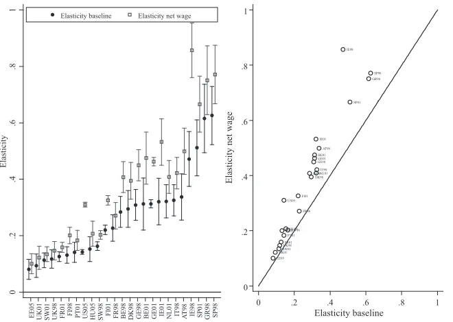
The size of hour elasticities might be infl uenced by differences in tax- benefi t systems across countries. Precisely, baseline elasticities are calculated by incrementing gross wages by 1 percent, as is common in the literature. Accordingly, the fact that high- tax countries are characterized by smaller net wage increments could explain smaller elas-ticities. To check this point, we simulate a 1 percent increase in the net wage in order to cancel out differences in effective marginal tax rates (EMTR) across countries due to different tax schedules or benefi t withdrawal rates. Figure 9 reports total hour elastici-ties in the baseline and this “net- wage increment” scenario. The right panel plots the two situations, while the left panel additionally indicates the 95 percent bootstrapped confi dence intervals. Elasticities after a 1 percent increase in net wage are generally larger; indeed, a 1 percent change in gross wages corresponds to smaller increments due to taxation. However, and most importantly, cross- country variation in elasticities is not truly affected when accounting for differences in implicit taxation of labor income.
C. Demographic Characteristics
We fi nally turn to the role of demographic composition. As indicated in Section III.B, important differences exist across countries in this respect, notably concerning the number of children yet also the age and education structure. Given that it is plausible
The Journal of Human Resources
EE05 UK01 PL05 SW01 FR01 FI98 PT01 US05 HU05 DK98 BE01 GE01 IE01 NL01 IT98 AT
9
8
SP01 GR98 Elasticity baseline Elasticity at mean levels
EE05
DK98BE01GE01IE01NL01 IT98
Elasticity at mean hour levels
0 .2 .4 .6 .8 1
DK98BE01GE01IE01NL01 IT98
Elasticity at mean wage levels
0 .2 .4 .6 .8 1
Elasticity baseline
Figure 8
that these demographic differences affect the size of mean elasticities, we decompose differences in elasticities across countries to investigate this point, using an approach similar to that in Heim (2007). Let i denote a woman’s age cohort, j her education group, and k the number of her children.31
Let εijk,c denote the wage elasticity of total hours for a woman of type ijk in country c. The mean elasticity in this country, εc, can be written as a weighted average ⌺i⌺j⌺kPijk,cεijk,c, where Pijk,c denotes the proportion of women of type ijk in this coun-try. This proportion can be rewritten as Pijk,c=Pi,cPj|i,cPk|ij,c where Pi,c denotes the proportion of women in age cohort i in country c, Pj|i,c the proportion of women in education group j given membership in age cohort i, and Pk|ij,c denotes the proportion of women with k children given membership in age cohort i and education group j. Letting P denote the mean proportion of a certain type over all countries, the propor-tion Pijk,c can be expressed as:
(8) Pijk,c=PiPj|iPk|ij+(Pi,c−Pi)Pj|iPk|ij+Pi,c(Pj|i,c−Pj|i)Pk|ij+Pi,cPj|i,c(Pk|ij,c−Pk|ij). This expression can be used to decompose the mean elasticity where εijk denotes the mean elasticity for type ijk over all countries:
31. In our application, we retain three age groups (aged 18–35, 36–45, and 45–59), two education groups, and three family sizes (no children, 1–2 children, and 3 children or more). Refi ning with three education groups leads to too many empty cells.
0
EE05 UK01 SW01 UK98 FR01 FI98 PT01 US05 HU05 SW98 FI01 FR98 BE98 DK98 GE98 BE01 GE01 IE01 NL01 IT98 AT
9
8
IE98 SP01 GR98 SP98 Elasticity baseline Elasticity net wage
EE05