An Introduction to Digital Image
Processing with
Matlab
Notes for SCM2511 Image
Processing 1
Semester 1, 2004
Alasdair McAndrew
School of Computer Science and Mathematics
Contents
1 Introduction 1
1.1 Images and pictures . . . 1
1.2 What is image processing? . . . 1
1.3 Image Acquisition and sampling . . . 4
1.4 Images and digital images . . . 8
1.5 Some applications . . . 10
1.6 Aspects of image processing . . . 11
1.7 An image processing task . . . 12
1.8 Types of digital images . . . 12
1.9 Image File Sizes . . . 14
1.10 Image perception . . . 16
1.11 Greyscale images . . . 17
1.12 RGB Images . . . 19
1.13 Indexed colour images . . . 21
1.14 Data types and conversions . . . 23
1.15 Basics of image display . . . 24
1.16 The imshowfunction . . . 26
1.17 Bit planes . . . 30
1.18 Spatial Resolution . . . 30
Exercises . . . 34
2 Point Processing 37 2.1 Introduction . . . 37
2.2 Arithmetic operations . . . 38
2.3 Histograms . . . 42
2.4 Lookup tables . . . 53
Exercises . . . 54
3 Neighbourhood Processing 57 3.1 Introduction . . . 57
3.2 Notation . . . 61
3.3 Filtering in Matlab . . . 62
3.4 Frequencies; low and high pass filters . . . 66
3.5 Edge sharpening . . . 70
3.6 Non-linear filters . . . 76
Exercises . . . 77
4.1 Introduction . . . 81
4.2 Background . . . 81
4.3 The one-dimensional discrete Fourier transform . . . 81
4.4 The two-dimensional DFT . . . 85
4.5 Fourier transforms inMatlab . . . 90
4.6 Fourier transforms of images . . . 92
4.7 Filtering in the frequency domain . . . 96
Exercises . . . 107
5 Image Restoration (1) 109 5.1 Introduction . . . 109
5.2 Noise . . . 110
5.3 Cleaning salt and pepper noise . . . 113
5.4 Cleaning Gaussian noise . . . 117
Exercises . . . 121
6 Image Restoration (2) 125 6.1 Removal of periodic noise . . . 125
6.2 Inverse filtering . . . 127
6.3 Wiener filtering . . . 132
Exercises . . . 133
7 Image Segmentation (1) 137 7.1 Introduction . . . 137
7.2 Thresholding . . . 137
7.3 Applications of thresholding . . . 140
7.4 Adaptive thresholding . . . 141
Exercises . . . 144
8 Image Segmentation (2) 145 8.1 Edge detection . . . 145
8.2 Derivatives and edges . . . 145
8.3 Second derivatives . . . 151
8.4 The Hough transform . . . 155
Exercises . . . 160
9 Mathematical morphology (1) 163 9.1 Introduction . . . 163
9.2 Basic ideas . . . 163
9.3 Dilation and erosion . . . 165
Exercises . . . 173
10 Mathematical morphology (2) 175 10.1 Opening and closing . . . 175
10.2 The hit-or-miss transform . . . 180
10.3 Some morphological algorithms . . . 182
11 Colour processing 191
11.1 What is colour? . . . 191
11.2 Colour models . . . 195
11.3 Colour images in Matlab . . . 199
11.4 Pseudocolouring . . . 202
11.5 Processing of colour images . . . 205
Exercises . . . 211
12 Image coding and compression 215 12.1 Lossless and lossy compression . . . 215
12.2 Huffman coding . . . 215
12.3 Run length encoding . . . 218
Exercises . . . 222
Bibliography 225
Introduction
1.1
Images and pictures
As we mentioned in the preface, human beings are predominantly visual creatures: we rely heavily on our vision to make sense of the world around us. We not only look at things to identify and classify them, but we can scan for differences, and obtain an overall rough “feeling” for a scene with a quick glance.
Humans have evolved very precise visual skills: we can identify a face in an instant; we can differentiate colours; we can process a large amount of visual information very quickly.
However, the world is in constant motion: stare at something for long enough and it will change in some way. Even a large solid structure, like a building or a mountain, will change its appearance depending on the time of day (day or night); amount of sunlight (clear or cloudy), or various shadows falling upon it.
We are concerned with single images: snapshots, if you like, of a visual scene. Although image processing can deal with changing scenes, we shall not discuss it in any detail in this text.
For our purposes, an image is a single picture which represents something. It may be a picture of a person, of people or animals, or of an outdoor scene, or a microphotograph of an electronic component, or the result of medical imaging. Even if the picture is not immediately recognizable, it will not be just a random blur.
1.2
What is image processing?
Image processing involves changing the nature of an image in order to either 1. improve its pictorial information for human interpretation,
2. render it more suitable for autonomous machine perception.
We shall be concerned withdigital image processing, which involves using a computer to change the nature of adigital image (see below). It is necessary to realize that these two aspects represent two separate but equally important aspects of image processing. A procedure which satisfies condition (1)—a procedure which makes an image “look better”—may be the very worst procedure for satis-fying condition (2). Humans like their images to be sharp, clear and detailed; machines prefer their images to be simple and uncluttered.
Examples of (1) may include:
Enhancing the edges of an image to make it appear sharper; an example is shown in figure 1.1. Note how the second image appears “cleaner”; it is a more pleasant image. Sharpening edges is a vital component of printing: in order for an image to appear “at its best” on the printed page; some sharpening is usually performed.
(a) The original image (b) Result after “sharperning”
Figure 1.1: Image sharperning
Removing “noise” from an image; noise being random errors in the image. An example is given in figure 1.2. Noise is a very common problem in data transmission: all sorts of electronic components may affect data passing through them, and the results may be undesirable. As we shall see in chapter 5 noise may take many different forms;each type of noise requiring a different method of removal.
Removing motion blur from an image. An example is given in figure 1.3. Note that in the deblurred image (b) it is easier to read the numberplate, and to see the spikes on the fence behind the car, as well as other details not at all clear in the original image (a). Motion blur may occur when the shutter speed of the camera is too long for the speed of the object. In photographs of fast moving objects: athletes, vehicles for example, the problem of blur may be considerable.
Examples of (2) may include:
(a) The original image (b) After removing noise
Figure 1.2: Removing noise from an image
(a) The original image (b) After removing the blur
From the edge result, we see that it may be necessary to enhance the original image slightly, to make the edges clearer.
(a) The original image (b) Its edge image
Figure 1.4: Finding edges in an image
Removing detail from an image. For measurement or counting purposes, we may not be interested in all the detail in an image. For example, a machine inspected items on an assembly line, the only matters of interest may be shape, size or colour. For such cases, we might want to simplify the image. Figure 1.5 shows an example: in image (a) is a picture of an African buffalo, and image (b) shows a blurred version in which extraneous detail (like the logs of wood in the background) have been removed. Notice that in image (b) all the fine detail is gone; what remains is the coarse structure of the image. We could for example, measure the size and shape of the animal without being “distracted” by unnecessary detail.
1.3
Image Acquisition and sampling
Sampling refers to the process of digitizing a continuous function. For example, suppose we take the function
✂✁☎✄✝✆✟✞✡✠☞☛✍✌✡✎✑✏
✒
✄✓✆✔✞✡✠
✒
☛✍✌✖✕
and sample it at ten evenly spaced values of ☛
(a) The original image (b) Blurring to remove detail
Figure 1.5: Blurring an image
Figure 1.6: Sampling a function—undersampling
✁ ✁ ✁ ✁ ✁ ✁ ✁ ✁ ✁ ✁ ✁ ✁ ✁ ✁ ✁ ✁ ✁ ✁✁ ✁ ✁ ✁ ✁ ✁ ✁ ✁ ✁✁ ✁ ✁ ✁ ✁ ✁ ✁ ✁ ✁ ✁ ✁ ✁ ✁ ✁ ✁ ✁ ✁ ✁✁ ✁ ✁ ✁ ✁ ✁ ✁ ✁ ✁✁ ✁ ✁ ✁ ✁ ✁ ✁ ✁ ✁✁ ✁ ✁ ✁ ✁ ✁ ✁ ✁ ✁ ✁ ✁ ✁ ✁ ✁ ✁ ✁ ✁ ✁✁ ✁ ✁ ✁ ✁ ✁ ✁ ✁ ✁✁ ✁ ✁ ✁ ✁ ✁ ✁ ✁ ✁ ✁
Sampling an image again requires that we consider the Nyquist criterion, when we consider an image as a continuous function of two variables, and we wish to sample it to produce a digital image. An example is shown in figure 1.8 where an image is shown, and then with an undersampled version. The jagged edges in the undersampled image are examples ofaliasing. The sampling rate
Correct sampling; no aliasing An undersampled version with aliasing
Figure 1.8: Effects of sampling
will of course affect the final resolution of the image; we discuss this below. In order to obtain a sampled (digital) image, we may start with a continuous representation of a scene. To view the scene, we record the energy reflected from it; we may use visible light, or some other energy source. Using light
Light is the predominant energy source for images; simply because it is the energy source which human beings can observe directly. We are all familiar with photographs, which are a pictorial record of a visual scene.
Many digital images are captured using visible light as the energy source; this has the advantage of being safe, cheap, easily detected and readily processed with suitable hardware. Two very popular methods of producing a digital image are with a digital camera or a flat-bed scanner.
CCD camera. Such a camera has, in place of the usual film, an array of photosites; these are silicon electronic devices whose voltage output is proportional to the intensity of light falling on them.
For a camera attached to a computer, information from the photosites is then output to a suitable storage medium. Generally this is done on hardware, as being much faster and more efficient than software, using aframe-grabbing card. This allows a large number of images to be captured in a very short time—in the order of one ten-thousandth of a second each. The images can then be copied onto a permanent storage device at some later time.
This is shown schematically in figure 1.9.
Original scene
CCD Array
Digital output
Figure 1.9: Capturing an image with a CCD array
Digital still cameras use a range of devices, from floppy discs and CD’s, to various specialized cards and “memory sticks”. The information can then be downloaded from these devices to a computer hard disk.
Flat bed scanner. This works on a principle similar to the CCD camera. Instead of the entire image being captured at once on a large array, a single row of photosites is moved across the image, capturing it row-by-row as it moves. Tis is shown schematically in figure 1.10.
M
ot
io
n
of
ro
w
Original scene
Output row
Output array
Row of photosites
Figure 1.10: Capturing an image with a CCD scanner
Since this is a much slower process than taking a picture with a camera, it is quite reasonable to allow all capture and storage to be processed by suitable software.
Other energy sources
the form of waves of varying wavelength. These range from cosmic rays of very short wavelength, to electric power, which has very long wavelength. Figure 1.11 illustrates this. For microscopy, we
Cosmic rays
Gamma
rays X-rays UV light
VISIBLE
LIGHT Infra-red
Micro-waves TV Radio
Electric Power
✂✁☎✄✝✆✟✞ ✂✁☎✄✝✆✠✆ ✂✁☎✄☛✡ ✂✁☎✄☛☞ ✌✎✍
✂✁☎✄☛✏ ✑
✍
✂✁☎✄☛✏✒✔✓✕
✍
✂✁☎✄☛✖✘✗
✍
✂✁☎✄✚✙ ✗
✍
✂✁☎✄✝✆ ✗✔✁ ✕
✍
✂✁✔✖
Blue Green Red
✛
✕
✒☛✜☛✢✤✣
✏
✥✝✦★✧☎✩ ✜
✕
✛✫✪
✏
✣
✏
✥✝✦★✧✬✩ ✭✮✣
✏
✥✝✦★✧✬✩
Figure 1.11: The electromagnetic spectrum
may use x-rays, or electron beams. As we can see from figure 1.11, x-rays have a shorter wavelength than visible light, and so can be used to resolve smaller objects than are possible with visible light. See Clark [2] for a good introduction to this. X-rays are of course also useful in determining the structure of objects usually hidden from view: such as bones.
A further method of obtaining images is by the use of x-ray tomography, where an object is encircled by an x-ray beam. As the beam is fired through the object, it is detected on the other side of the object, as shown in figure 1.12. As the beam moves around the object, an image of the object can be constructed; such an image is called atomogram. In a CAT (Computed Axial Tomography) scan, the patient lies within a tube around which x-ray beams are fired. This enables a large number of tomographic “slices” to be formed, which can then be joined to produce a three-dimensional image. A good account of such systems (and others) is given by Siedband [13]
1.4
Images and digital images
Suppose we take an image, a photo, say. For the moment, lets make things easy and suppose the photo is monochromatic (that is, shades of grey only), so no colour. We may consider this image as being a two dimensional function, where the function values give the brightness of the image at any given point, as shown in figure 1.13. We may assume that in such an image brightness values can be any real numbers in the range ✥
✕
✥
(black) to ✏
✕
✥
(white). The ranges of ☛
and will clearly depend on the image, but they can take all real values between their minima and maxima.
Object X-ray source
Object
Detectors
Figure 1.12: X-ray tomography
☛
✠☞☛✂✁ ✌ ✁
✥
✕
✢
be vital for the development and implementation of image processing techniques.
Figure 1.14: The image of figure 1.13 plotted as a function of two variables
A digital image differs from a photo in that the ☛
, , and ✠☞☛✂✁ ✌
values are alldiscrete. Usually they take on only integer values, so the image shown in figure 1.13 will have ☛
and ranging from 1 to 256 each, and the brightness values also ranging from 0 (black) to 255 (white). A digital image, as we have seen above, can be considered as a large array of sampled points from the continuous image, each of which has a particular quantized brightness; these points are thepixels which constitute the digital image. The pixels surrounding a given pixel constitute its neighbourhood. A neighbourhood can be characterized by its shape in the same way as a matrix: we can speak, for example, of a✒ ✣ ✒ neighbourhood, or of a ✜ ✣ ✭
neighbourhood. Except in very special circumstances, neighbourhoods have odd numbers of rows and columns; this ensures that the current pixel is in the centre of the neighbourhood. An example of a neighbourhood is given in figure 1.15. If a neighbourhood has an even number of rows or columns (or both), it may be necessary to specify which pixel in the neighbourhood is the “current pixel”.
1.5
Some applications
Image processing has an enormous range of applications; almost every area of science and technology can make use of image processing methods. Here is a short list just to give some indication of the range of image processing applications.
48 219 168 145 244 188 120 58
49 218 87 94 133 35 17 148
174 151 74 179 224 3 252 194
77 127 87 139 44 228 149 135
138 229 136 113 250 51 108 163
38 210 185 177 69 76 131 53
178 164 79 158 64 169 85 97
96 209 214 203 223 73 110 200
Current pixel
✒ ✣ ✜
neighbourhood
Figure 1.15: Pixels, with a neighbourhood
Inspection and interpretation of images obtained from X-rays, MRI or CAT scans, analysis of cell images, of chromosome karyotypes.
2. Agriculture
Satellite/aerial views of land, for example to determine how much land is being used for different purposes, or to investigate the suitability of different regions for different crops, inspection of fruit and vegetables—distinguishing good and fresh produce from old. 3. Industry
Automatic inspection of items on a production line, inspection of paper samples.
4. Law enforcement
Fingerprint analysis,
sharpening or de-blurring of speed-camera images.
1.6
Aspects of image processing
It is convenient to subdivide different image processing algorithms into broad subclasses. There are different algorithms for different tasks and problems, and often we would like to distinguish the nature of the task at hand.
Image enhancement. This refers to processing an image so that the result is more suitable for a particular application. Example include:
sharpening or de-blurring an out of focus image, highlighting edges,
removing noise.
Image restoration. This may be considered as reversing the damage done to an image by a known cause, for example:
removing of blur caused by linear motion, removal of optical distortions,
removing periodic interference.
Image segmentation. This involves subdividing an image into constituent parts, or isolating certain aspects of an image:
finding lines, circles, or particular shapes in an image,
in an aerial photograph, identifying cars, trees, buildings, or roads.
These classes are not disjoint; a given algorithm may be used for both image enhancement or for image restoration. However, we should be able to decide what it is that we are trying to do with our image: simply make it look better (enhancement), or removing damage (restoration).
1.7
An image processing task
We will look in some detail at a particular real-world task, and see how the above classes may be used to describe the various stages in performing this task. The job is to obtain, by an automatic process, the postcodes from envelopes. Here is how this may be accomplished:
Acquiring the image. First we need to produce a digital image from a paper envelope. This an be done using either a CCD camera, or a scanner.
Preprocessing. This is the step taken before the “major” image processing task. The problem here is to perform some basic tasks in order to render the resulting image more suitable for the job to follow. In this case it may involve enhancing the contrast, removing noise, or identifying regions likely to contain the postcode.
Segmentation. Here is where we actually “get” the postcode; in other words we extract from the image that part of it which contains just the postcode.
Representation and description. These terms refer to extracting the particular features which allow us to differentiate between objects. Here we will be looking for curves, holes and corners which allow us to distinguish the different digits which constitute a postcode.
Recognition and interpretation. This means assigning labels to objects based on their descrip-tors (from the previous step), and assigning meanings to those labels. So we identify particular digits, and we interpret a string of four digits at the end of the address as the postcode.
1.8
Types of digital images
Binary. Each pixel is just black or white. Since there are only two possible values for each pixel, we only need one bit per pixel. Such images can therefore be very efficient in terms of storage. Images for which a binary representation may be suitable include text (printed or handwriting), fingerprints, or architectural plans.
An example was the image shown in figure 1.4(b) above. In this image, we have only the two colours: white for the edges, and black for the background. See figure 1.16 below.
1 1 0 0 0 0
0 0 1 0 0 0
0 0 1 0 0 0
0 0 0 1 0 0
0 0 0 1 1 0
0 0 0 0 0 1
Figure 1.16: A binary image
Greyscale. Each pixel is a shade of grey, normally from ✥
(black) to ✜☛✜
(white). This range means that each pixel can be represented by eight bits, or exactly one byte. This is a very natural range for image file handling. Other greyscale ranges are used, but generally they are a power of 2. Such images arise in medicine (X-rays), images of printed works, and indeed
✜ ✪
different grey levels is sufficient for the recognition of most natural objects. An example is the street scene shown in figure 1.1 above, and in figure 1.17 below.
True colour, or RGB. Here each pixel has a particular colour; that colour being described by the amount of red, green and blue in it. If each of these components has a range✥
– ✜☛✜
, this gives a total of ✜☛✜
✗
✁
✏
✪
✁
✭☛✭☛✭
✁
✏
✪
different possible colours in the image. This is enough colours for any image. Since the total number of bits required for each pixel is ✛
, such images are also called ✛
-bit colour images.
Such an image may be considered as consisting of a “stack” of three matrices; representing the red, green and blue values for each pixel. This means that for every pixel there correspond three values.
An example is shown in figure 1.18.
230 229 232 234 235 232 148
237 236 236 234 233 234 152
255 255 255 251 230 236 161
99 90 67 37 94 247 130
222 152 255 129 129 246 132
154 199 255 150 189 241 147
216 132 162 163 170 239 122
Figure 1.17: A greyscale image
or colour palette, which is simply a list of all the colours used in that image. Each pixel has a value which does not give its colour (as for an RGB image), but anindex to the colour in the map.
It is convenient if an image has ✜ ✪
colours or less, for then the index values will only require one byte each to store. Some image file formats (for example, Compuserve GIF), allow only
✜
✪
colours or fewer in each image, for precisely this reason.
Figure 1.19 shows an example. In this image the indices, rather then being the grey values of the pixels, are simply indices into the colour map. Without the colour map, the image would be very dark and colourless. In the figure, for example, pixels labelled5 correspond to 0.2627 0.2588 0.2549, which is a dark greyish colour.
1.9
Image File Sizes
Image files tend to be large. We shall investigate the amount of information used in different image type of varying sizes. For example, suppose we consider a ✜
✏
✣ ✜
✏ binary image. The number of bits used in this image (assuming no compression, and neglecting, for the sake of discussion, any header information) is
✜
✏
✣ ✜
✏
✣
✏
✁
✪
✁
✏
✛☛✛
✁
Red Green Blue 49 55 56 57 52 53
58 60 60 58 55 57
58 58 54 53 55 56
83 78 72 69 68 69
88 91 91 84 83 82
69 76 83 78 76 75
61 69 73 78 76 76
64 76 82 79 78 78
93 93 91 91 86 86
88 82 88 90 88 89
125 119 113 108 111 110
137 136 132 128 126 120
105 108 114 114 118 113
96 103 112 108 111 107
66 80 77 80 87 77
81 93 96 99 86 85
83 83 91 94 92 88
135 128 126 112 107 106
141 129 129 117 115 101
95 99 109 108 112 109
84 93 107 101 105 102
4 5 5 5 5 5
5 4 5 5 6 6
5 5 5 0 8 9
5 5 5 5 11 11
5 5 5 8 16 20
8 11 11 26 33 20
11 20 33 33 58 37
0.1211 0.1211 0.1416
0.1807 0.2549 0.1729
0.2197 0.3447 0.1807
0.1611 0.1768 0.1924
0.2432 0.2471 0.1924
0.2119 0.1963 0.2002
0.2627 0.2588 0.2549
0.2197 0.2432 0.2588 .
.
. ... ...
Indices
Colour map
Figure 1.19: An indexed colour image
✁ ✒ ✕ ✭ ✪ ✢ Kb ✥ ✕ ✥ ✒ ✒ Mb.
(Here we use the convention that a kilobyte is one thousand bytes, and a megabyte is one million bytes.)
A greyscale image of the same size requires:
✜ ✏ ✣ ✜ ✏ ✣ ✏ ✁ ✪ ✁ ✏ ✛☛✛ bytes ✁ ✪ ✕ ✏ ✛ Kb ✥ ✕ ✪ Mb.
If we now turn our attention to colour images, each pixel is associated with 3 bytes of colour information. A ✜
✏
✣ ✜
✏ image thus requires
✜ ✏ ✣ ✜ ✏ ✣ ✒ ✁ ✭ ✢ ✪ ✁ ✛ ✒ bytes ✁ ✭ ✢ ✪ ✕ ✛ ✒ Kb ✥ ✕ ✭ ✢ ✪ Mb.
Many images are of course such larger than this; satellite images may be of the order of several thousand pixels in each direction.
1.10
Image perception
Much of image processing is concerned with making an image appear “better” to human beings. We should therefore be aware of the limitations of the the human visual system. Image perception consists of two basic steps:
2. recognising and interpreting the image with thevisual cortex in the brain.
The combination and immense variability of these steps influences the ways in we perceive the world around us.
There are a number of things to bear in mind:
1. Observed intensities vary as to the background. A single block of grey will appear darker if placed on a white background than if it were placed on a black background. That is, we don’t perceive grey scales “as they are”, but rather as they differ from their surroundings. In figure 1.20 a grey square is shown on two different backgrounds. Notice how much darker the square appears when it is surrounded by a light grey. However, the two central squares have exactly the same intensity.
Figure 1.20: A grey square on different backgrounds
2. We may observe non-existent intensities as bars in continuously varying grey levels. See for example figure 1.21. This image varies continuously from light to dark as we travel from left to right. However, it is impossible for our eyes not to see a few horizontal edges in this image. 3. Our visual system tends to undershoot or overshoot around the boundary of regions of different intensities. For example, suppose we had a light grey blob on a dark grey background. As our eye travels from the dark background to the light region, the boundary of the region appears lighter than the rest of it. Conversely, going in the other direction, the boundary of the background appears darker than the rest of it.
We have seen in the previous chapter that matrices can be handled very efficiently in Matlab. Images may be considered as matrices whose elements are the pixel values of the image. In this chapter we shall investigate how the matrix capabilities of Matlab allow us to investigate images and their properties.
1.11
Greyscale images
Suppose you are sitting at your computer and have started Matlab. You will have a Matlab
Figure 1.21: Continuously varying intensities
>>
ready to receive commands. Type in the command >> w=imread(’wombats.tif’);
This takes the grey values of all the pixels in the greyscale image wombats.tif and puts them all into a matrix w. This matrix w is now a Matlab variable, and so we can perform various matrix operations on it. In general the imread function reads the pixel values from an image file, and returns a matrix of all the pixel values.
Two things to note about this command:
1. It ends in asemicolon; this has the effect of not displaying the results of the command to the screen. As the result of this particular command is a matrix of size ✜
✪
✣ ✜
✪
, or with ✪ ✜☛✜ ✒
✪
elements, we don’t really want all its values displayed.
2. The namewombats.tifis given in single quote marks. Without them,Matlabwould assume thatwombats.tifwas the name of a variable, rather than the name of a file.
Now we can display this matrix as a greyscale image: >> figure,imshow(w),pixval on
This is really three commands on the one line. Matlab allows many commands to be entered on the same line; using commas to separate the different commands. The three commands we are using here are:
figure, which creates a figure on the screen. A figure is a window in which a graphics object can be placed. Objects may include images, or various types of graphs.
pixval on, which turns on the pixel values in our figure. This is a display of the grey values of the pixels in the image. They appear at the bottom of the figure in the form
✣✂✁ ✁☎✄
where is the column value of the given pixel; ✁
its row value, and ✄
its grey value. Since wombats.tif is an 8-bit greyscale image, the pixel values appear as integers in the range
✥
– ✜☛✜ .
This is shown in figure 1.22.
Figure 1.22: The wombats image withpixval on
If there are no figures open, then an imshowcommand, or any other command which generates a graphics object, will open a new figure for displaying the object. However, it is good practice to use thefigurecommand whenever you wish to create a new figure.
We could display this image directly, without saving its grey values to a matrix, with the command
imshow(’wombats.tif’)
However, it is better to use a matrix, seeing as these are handled very efficiently inMatlab.
1.12
RGB Images
in fact a number of different methods for describing colour, but for image display and storage a standard model is RGB, for which we may imagine all the colours sitting inside a “colour cube” of side ✏ as shown in figure 1.23. The colours along the black-white diagonal, shown in the diagram
✁ ✂ ✄ ☎ ✆ ✠ ✥ ✁ ✥ ✁ ✥ ✌ Black ✠ ✏ ✁ ✥ ✁ ✥ ✌ Red ✠ ✥ ✁ ✏ ✁ ✥ ✌ Green ✠ ✥ ✁ ✥ ✁ ✏ ✌ Blue ✠ ✏ ✁ ✥ ✁ ✏ ✌ Magenta ✠ ✏ ✁ ✏ ✁ ✥ ✌ Yellow ✠ ✥ ✁ ✏ ✁ ✏ ✌ Cyan ✠ ✏ ✁ ✏ ✁ ✏ ✌ White
Figure 1.23: The colour cube for the RGB colour model
as a dotted line, are the points of the space where all the ✄ , ✆
, ☎
values are equal. They are the different intensities of grey. We may also think of the axes of the colour cube as being discretized to integers in the range 0–255.
RGB is the standard for thedisplay of colours: on computer monitors; on TV sets. But it is not a very good way ofdescribing colours. How, for example, would you define light brown using RGB? As we shall see also in chapter 11, there are some colours which are not realizable with the RGB model; in that they would require negative values of one or two of the RGB components. Matlab
handles 24-bit RGB images in much the same way as greyscale. We can save the colour values to a matrix and view the result:
>> a=imread(’autumn.tif’); >> figure,imshow(a),pixval on
Note now that the pixel values now consist of a list of three values, giving the red, green and blue components of the colour of the given pixel.
An important difference between this type of image and a greyscale image can be seen by the command
>> size(a)
which returns three values: the number of rows, columns, and “pages” of a, which is a three-dimensional matrix, also called a multidimensional array. Matlab can handle arrays of any di-mension, and a is an example. We can think of a as being a stack of three matrices, each of the same size.
>> a(100,200,2)
returns the second colour value (green) at the pixel in row 100 and column 200. If we want all the colour values at that point, we can use
>> a(100,200,1:3)
However, Matlab allows a convenient shortcut for listing all values along a particular dimension; just using a colon on its own:
>> a(100,200,:)
A useful function for obtaining RGB values is impixel; the command >> impixel(a,200,100)
returns the red, green, and blue values of the pixel at column 200, row 100. Notice that the order of indexing is the same as that which is provided by the pixval oncommand. This is opposite to the row, column order for matrix indexing. This command also applies to greyscale images:
>> impixel(g,100,200)
will return three values, but since g is a single two-dimensional matrix, all three values will be the same.
1.13
Indexed colour images
The command
>> figure,imshow(’emu.tif’),pixval on
produces a nice colour image of an emu. However, the pixel values, rather than being three integers as they were for the RGB image above, are three fractions between 0 and 1. What is going on here?
If we try saving to a matrix first and then displaying the result: >> em=imread(’emu.tif’);
>> figure,imshow(em),pixval on
we obtain a dark, barely distinguishable image, with single integer grey values, indicating that em is being interpreted as a single greyscale image.
In fact the image emu.tif is an example of an indexed image, consisting of two matrices: a colour map, and anindex to the colour map. Assigning the image to a single matrix picks up only the index; we need to obtain the colour map as well:
>> [em,emap]=imread(’emu.tif’); >> figure,imshow(em,emap),pixval on
Information about your image
A great deal of information can be obtained with the imfinfo function. For example, suppose we take our indexed image emu.tif from above.
>> imfinfo(’emu.tif’)
ans =
Filename: ’emu.tif’
FileModDate: ’26-Nov-2002 14:23:01’ FileSize: 119804
Format: ’tif’ FormatVersion: []
Width: 331 Height: 384 BitDepth: 8
ColorType: ’indexed’ FormatSignature: [73 73 42 0]
ByteOrder: ’little-endian’ NewSubfileType: 0
BitsPerSample: 8
Compression: ’PackBits’ PhotometricInterpretation: ’RGB Palette’
StripOffsets: [16x1 double] SamplesPerPixel: 1
RowsPerStrip: 24
StripByteCounts: [16x1 double] XResolution: 72
YResolution: 72 ResolutionUnit: ’Inch’
Colormap: [256x3 double] PlanarConfiguration: ’Chunky’
TileWidth: [] TileLength: [] TileOffsets: [] TileByteCounts: [] Orientation: 1
FillOrder: 1 GrayResponseUnit: 0.0100
MaxSampleValue: 255 MinSampleValue: 0
Thresholding: 1
For comparison, let’s look at the output of a true colour file (showing only the first few lines of the output):
>> imfinfo(’flowers.tif’)
ans =
Filename: [1x57 char]
FileModDate: ’26-Oct-1996 02:11:09’ FileSize: 543962
Format: ’tif’ FormatVersion: []
Width: 500 Height: 362 BitDepth: 24
ColorType: ’truecolor’
Now we shall test this function on a binary image: >> imfinfo(’text.tif’)
ans =
Filename: [1x54 char]
FileModDate: ’26-Oct-1996 02:12:23’ FileSize: 3474
Format: ’tif’ FormatVersion: []
Width: 256 Height: 256 BitDepth: 1
ColorType: ’grayscale’
What is going on here? We have a binary image, and yet the colour type is given as “grayscale”. The fact is thatMatlabdoes not distinguish between greyscale and binary images: a binary image is just a special case of a greyscale image which has only two intensities. However, we can see that text.tifis a binary image since the number of bits per pixel is only one.
1.14
Data types and conversions
Elements inMatlabmatrices may have a number of different numeric data types; the most common are listed in table 1.1. There are others, but those listed will be sufficient for all our work with images. These data types are also functions, we can convert from one type to another. For example:
>> a=23; >> b=uint8(a); >> b
Data type Description Range
int8 8-bit integer ✏
✢
— 127
uint8 8-bit unsigned integer 0 — 255
int16 16-bit integer ✒ ✭ ✪ ✢
— 32767
uint16 16-bit unsigned integer 0 — 65535
double Double precision real number Machine specific
Table 1.1: Data types inMatlab
23
>> whos a b
Name Size Bytes Class
a 1x1 8 double array
b 1x1 1 uint8 array
Even though the variablesaandbhave the same numeric value, they are of different data types. An important consideration (of which we shall more) is that arithmetic operations are not permitted with the data typesint8,int16,uint8and uint16.
A greyscale image may consist of pixels whose values are of data type uint8. These images are thus reasonably efficient in terms of storage space, since each pixel requires only one byte. However, arithmetic operations are not permitted on this data type; a uint8 image must be converted to doublebefore any arithmetic is attempted.
We can convert images from one image type to another. Table 1.2 lists all ofMatlab’s functions for converting between different image types. Note that the gray2rgb function, does not create a
Function Use Format
ind2gray Indexed to Greyscale y=ind2gray(x,map); gray2ind Greyscale to indexed [y,map]=gray2ind(x); rgb2gray RGB to greyscale y=rgb2gray(x);
gray2rgb Greyscale to RGB y=gray2rgb(x); rgb2ind RGB to indexed [y,map]=rgb2ind; ind2rgb Indexed to RGB y=ind2rgb(x,map);
Table 1.2: Converting images inMatlab
colour image, but an image all of whose pixel colours were the same as before. This is done by simply replicating the grey values of each pixel: greys in an RGB image are obtained by equality of the red, green and blue values.
1.15
Basics of image display
they include:
1. ambient lighting,
2. the monitor type and settings, 3. the graphics card,
4. monitor resolution.
The same image may appear very different when viewed on a dull CRT monitor or on a bright LCD monitor. The resolution can also affect the display of an image; a higher resolution may result in the image taking up less physical area on the screen, but this may be counteracted by a loss in the colour depth: the monitor may be only to display 24-bit colour at low resolutions. If the monitor is bathed in bright light (sunlight, for example), the display of the image may be compromised. Furthermore, the individual’s own visual system will affect the appearance of an image: the same image, viewed by two people, may appear to have different characteristics to each person. For our purpose, we shall assume that the computer set up is as optimal as is possible, and the monitor is able to accurately reproduce the necessary grey values or colours in any image.
A very basic Matlab function for image display is image. This function simply displays a matrix as an image. However, it may not give necessarily very good results. For example:
>> c=imread(’cameraman.tif’); >> image(c)
will certainly display the cameraman, but possibly in an odd mixture of colours, and with some stretching. The strange colours come from the fact that theimagecommand uses the current colour map to assign colours to the matrix elements. The default colour map is calledjet, and consists of 64 very bright colours, which is inappropriate for the display of a greyscale image.
To display the image properly, we need to add several extra commands to the image line. 1. truesize, which displays one matrix element (in this case an image pixel) for each screen
pixel. More formally, we may use truesize([256 256])where the vector components give the number of screen pixels vertically and horizontally to use in the display. If the vector is not specified, it defaults to the image size.
2. axis offwhich turns off the axis labelling,
3. colormap(gray(247)), which adjusts the image colour map to use shades of grey only. We can find the number of grey levels used by the cameraman image with
>> size(unique(c))
ans =
247 1
Since the cameraman image thus uses 247 different grey levels, we only need that number of greys in the colour map.
>> image(c),truesize,axis off, colormap(gray(247))
We may to adjust the colour map to use less or more colours; however this can have a dramatic effect on the result. The command
>> image(c),truesize,axis off, colormap(gray(512))
will produce a dark image. This happens because only the first 247 elements of the colour map will be used by the image for display, and these will all be in the first half of the colour map; thus all dark greys. On the other hand,
>> image(c),truesize,axis off, colormap(gray(128))
will produce a very light image, because any pixel with grey level higher than 128 will simply pick that highest grey value (which is white) from the colour map.
The image command works well for an indexed colour image, as long as we remember to use imreadto pick up the colour map as well:
>> [x,map]=imread(’cat.tif’);
>> image(x),truesize,axis off,colormap(map)
For true colour images, the image data will be read (by imread) as a three dimensional array. In such a case, image will ignore the current colour map, and assign colours to the display based on the values in the array. So
>> t=imread(’twins.tif’); >> image(t),truesize,axis off
will produce the correct twins image.
In general the image function can be used to display any image or matrix. However, there is a command which is more convenient, and does most of the work of colour mapping for us; we discuss this in the next section.
1.16
The
imshow
function
Greyscale images
We have seen that if x is a matrix of typeuint8, then the command imshow(x)
will display x as an image. This is reasonable, since the data type uint8 restricts values to be integers between 0 and 255. However, not all image matrices come so nicely bundled up into this data type, and lots of Matlab image processing commands produces output matrices which are of typedouble. We have two choices with a matrix of this type:
The second option is possible because imshowwill display a matrix of type double as a greyscale image as long as the matrix elements are between 0 and 1. Suppose we take an image and convert it to type double:
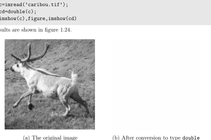
>> c=imread(’caribou.tif’); >> cd=double(c);
>> imshow(c),figure,imshow(cd)
The results are shown in figure 1.24.
[image:31.595.105.516.119.392.2](a) The original image (b) After conversion to type double
Figure 1.24: An attempt at data type conversion
However, as you can see, figure 1.24(b) doesn’t look much like the original picture at all! This is because for a matrix of typedouble, theimshowfunction expects the values to be between 0 and 1, where 0 is displayed as black, and 1 is displayed as white. A value with ✥✂✁ ✁
✏ is displayed as grey scale ✄
✜☛✜ ✆☎
. Conversely, values greater than 1 will be displayed as 1 (white) and values less than 0 will be displayed as zero (black). In the caribou image, every pixel has value greater than or equal to 1 (in fact the minimum value is 21), so that every pixel will be displayed as white. To display the matrixcd, we need to scale it to the range 0—1. This is easily done simply by dividing all values by 255:
>> imshow(cd/255)
and the result will be the caribou image as shown in figure 1.24(a).
We can vary the display by changing the scaling of the matrix. Results of the commands: >> imshow(cd/512)
>> imshow(cd/128)
are shown in figures 1.25.
(a) The matrixcddivided by 512 (b) The matrix cddivided by 128
Figure 1.25: Scaling by dividing an image matrix by a scalar
The display of the result of a command whose output is a matrix of type doublecan be greatly affected by a judicious choice of a scaling factor.
We can convert the original image todoublemore properly using the functionim2double. This applies correct scaling so that the output values are between 0 and 1. So the commands
>> cd=im2double(c); >> imshow(cd)
will produce a correct image. It is important to make the distinction between the two functions double and im2double: double changes the data type but does not change the numeric values; im2double changes both the numeric data type and the values. The exception of course is if the original image is of type double, in which case im2double does nothing. Although the command doubleis not of much use for direct image display, it can be very useful for image arithmetic. We have seen examples of this above with scaling.
Corresponding to the functions double andim2double are the functions uint8 and im2uint8. If we take our image cd of typedouble, properly scaled so that all elements are between 0 and 1, we can convert it back to an image of type uint8in two ways:
>> c2=uint8(255*cd); >> c3=im2uint8(cd);
Use of im2uint8is to be preferred; it takes other data types as input, and always returns a correct result.
Binary images
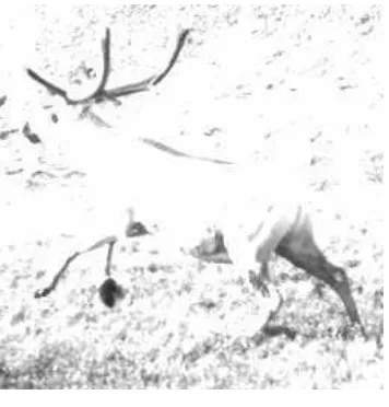
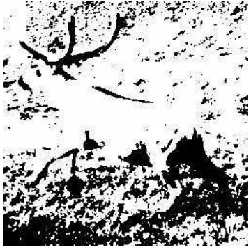
>> cl=c>120;
(we will see more of this type of operation in chapter 2.) If we now check all of our variables with whos, the output will include the line:
cl 256x256 65536 uint8 array (logical)
This means that the command >> imshow(cl)
will display the matrix as a binary image; the result is shown in figure 1.26.
[image:33.595.112.292.230.411.2](a) The caribou image turned binary (b) After conversion to typeuint8
Figure 1.26: Making the image binary
Suppose we remove the logical flag from cl; this can be done by a simple command: >> cl = +cl;
Now the output of whoswill include the line:
cl 256x256 65536 uint8 array
If we now try to display this matrix with imshow, we obtain the result shown in figure 1.26(b). A very disappointing image! But this is to be expected; in a matrix of typeuint8, white is 255, 0 is black, and 1 is a very dark grey–indistinguishable from black.
To get back to a viewable image, we can either turn the logical flag back on, and the view the result:
>> imshow(logical(cl))
or simply convert to type double: >> imshow(double(cl))
1.17
Bit planes
Greyscale images can be transformed into a sequence of binary images by breaking them up into theirbit-planes. If we consider the grey value of each pixel of an 8-bit image as an 8-bit binary word, then the 0th bit plane consists of the last bit of each grey value. Since this bit has the least effect in terms of the magnitude of the value, it is called the least significant bit, and the plane consisting of those bits the least significant bit plane. Similarly the 7th bit plane consists of the first bit in each value. This bit has the greatest effect in terms of the magnitude of the value, so it is called the most significant bit, and the plane consisting of those bits themost significant bit plane.
If we take a greyscale image, we start by making it a matrix of typedouble; this means we can perform arithmetic on the values.
>> c=imread(’cameraman.tif’); >> cd=double(c);
We now isolate the bit planes by simply dividing the matrix cdby successive powers of 2, throwing away the remainder, and seeing if the final bit is 0 or 1. We can do this with themod function.
>> c0=mod(cd,2);
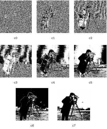
>> c1=mod(floor(cd/2),2); >> c2=mod(floor(cd/4),2); >> c3=mod(floor(cd/8),2); >> c4=mod(floor(cd/16),2); >> c5=mod(floor(cd/32),2); >> c6=mod(floor(cd/64),2); >> c7=mod(floor(cd/128),2);
These are all shown in figure 1.27. Note that the least significant bit plane,c0, is to all intents and purposes a random array, and that as the index value of the bit plane increases, more of the image appears. The most significant bit plane, c7, is actually athreshold of the image at level 127:
>> ct=c>127;
>> all(c7(:)==ct(:))
ans =
1
We shall discuss thresholding in chapter 7.
We can recover and display the original image with
>> cc=2*(2*(2*(2*(2*(2*(2*c7+c6)+c5)+c4)+c3)+c2)+c1)+c0; >> imshow(uint8(cc))
1.18
Spatial Resolution
c0 c1 c2
c3 c4 c5
[image:35.595.134.481.169.588.2]c6 c7
imresize function. Suppose we have an ✜ ✪ ✣ ✜ ✪
8-bit greyscale image saved to the matrix x. Then the command
imresize(x,1/2);
will halve the size of the image. It does this by taking out every other row and every other column, thus leaving only those matrix elements whose row and column indices are even:
☛ ✔ ☛ ✁ ☛ ✂✗ ☛ ✌ ☛ ✂✕ ☛ ✁✂ ✕ ✕ ✕ ☛ ☎ ☛ ✄ ☛ ✔✗ ☛ ✌ ☛ ✔✕ ☛ ✄✂ ✕ ✕ ✕ ☛ ✗☎ ☛ ✗✄ ☛ ✗✔✗ ☛ ✗ ✌ ☛ ✗✔✕ ☛ ✗✄✂ ✕ ✕ ✕ ☛ ✌ ☛ ✌ ☛ ✌ ✗ ☛ ✌✔✌ ☛ ✌ ✕ ☛ ✌ ✂ ✕ ✕ ✕ ☛ ✕☎ ☛ ✕✄ ☛ ✕✔✗ ☛ ✕ ✌ ☛ ✕✔✕ ☛ ✕✄✂ ✕ ✕ ✕ ☛ ✂☎ ☛ ✂✄ ☛ ✂✔✗ ☛ ✂ ✌ ☛ ✂✔✕ ☛ ✂✄✂ ✕ ✕ ✕ .. . ... ... ... ... ... . ..
✆☎ imresize(x,1/2) ✝☎
☛ ✄ ☛ ✌ ☛ ✄✂ ✕ ✕ ✕ ☛ ✌ ☛ ✌✔✌ ☛ ✌ ✂ ✕ ✕ ✕ ☛ ✂✄ ☛ ✂ ✌ ☛ ✂✄✂ ✕ ✕ ✕ .. . ... ... . ..
If we applyimresizeto the result with the parameter2 rather than1/2, all the pixels are repeated to produce an image with the same size as the original, but with half the resolution in each direction:
☛ ✄ ☛ ✄ ☛ ✄ ☛ ✄ ☛ ✌ ☛ ✌ ☛ ✌ ☛ ✌ ☛ ✄✂ ☛ ✄✂ ☛ ✄✂ ☛ ✄✂ ✕ ✕ ✕ ☛ ✌ ☛ ✌ ☛ ✌ ☛ ✌ ☛ ✌✔✌ ☛ ✌✔✌ ☛ ✌✔✌ ☛ ✌✔✌ ☛ ✌ ✂ ☛ ✌ ✂ ☛ ✌ ✂ ☛ ✌ ✂ ✕ ✕ ✕ ☛ ✂✄ ☛ ✂✄ ☛ ✂✄ ☛ ✂✄ ☛ ✂ ✌ ☛ ✂ ✌ ☛ ✂ ✌ ☛ ✂ ✌ ☛ ✂✄✂ ☛ ✂✄✂ ☛ ✂✄✂ ☛ ✂✄✂ ✕ ✕ ✕ .. . ... ... . ..
The effective resolution of this new image is only ✏ ✢ ✣
✏
✢
. We can do all this in one line: x2=imresize(imresize(x,1/2),2);
By changing the parameters of imresize, we can change the effective resolution of the image to smaller amounts:
Command Effective resolution
imresize(imresize(x,1/4),4); ✪ ✛ ✣ ✪ ✛ imresize(imresize(x,1/8),8); ✒ ✣ ✒ imresize(imresize(x,1/16),16); ✏
✪ ✣
✏
✪
imresize(imresize(x,1/32),32); ✢✮✣ ✢
To see the effects of these commands, suppose we apply them to the imagenewborn.tif: x=imread(’newborn.tif’);
The effects of increasing blockiness or pixelization become quite pronounced as the resolution de-creases; even at ✏
✢ ✣
✏
✢
resolution fine detail, such as the edges of the baby’s fingers, are less clear, and at ✪ ✛ ✣ ✪ ✛
all edges are now quite blocky. At ✒ ✣ ✒
the image is barely recognizable, and at ✪ ✣ ✪
and ✢ ✣ ✢
(a) The original image (b) at ✏ ✢ ✣
✏
✢
resolution
Figure 1.28: Reducing resolution of an image
(a) At ✪ ✛ ✣ ✪ ✛
resolution (b) At ✒ ✣ ✒
resolution
(a) At ✏
✪
✣
✏
✪
resolution (b) at ✢✮✣ ✢
resolution
Figure 1.30: Even more reducing the resolution of an image
Exercises
1. Watch the TV news, and see if you can observe any examples of image processing.
2. If your TV set allows it, turn down the colour as far as you can to produce a monochromatic display. How does this affect your viewing? Is there anything which is hard to recognize without colour?
3. Look through a collection of old photographs. How can they be enhanced, or restored? 4. For each of the following, list five ways in which image processing could be used:
medicine astronomy sport music agriculture travel
5. Image processing techniques have become a vital part of the modern movie production process. Next time you watch a film, take note of all the image processing involved.
6. If you have access to a scanner, scan in a photograph, and experiment with all the possible scanner settings.
(a) What is the smallest sized file you can create which shows all the detail of your photo-graph?
(c) How do the colour settings affect the output?
7. If you have access to a digital camera, again photograph a fixed scene, using all possible camera settings.
(a) What is the smallest file you can create? (b) How do the light settings effect the output?
8. Suppose you were to scan in a monochromatic photograph, and then print out the result. Then suppose you scanned in the printout, and printed out the result of that, and repeated this a few times. Would you expect any degradation of the image during this process? What aspects of the scanner and printer would minimize degradation?
9. Look up ultrasonography. How does it differ from the image acquisition methods discussed in this chapter? What is it used for? If you can, compare an ultrasound image with an x-ray image. How to they differ? In what ways are they similar?
10. If you have access to an image viewing program (other than Matlab) on your computer, make a list of the image processing capabilities it offers. Can you find imaging tasks it is unable to do?
11. Type in the command >> help imdemos
This will give you a list of, amongst other things, all the sample TIFF images which come with the Image Processing Toolbox. Make a list of these sample images, and for each image
(a) determine its type (binary, greyscale, true colour or indexed colour), (b) determine its size (in pixels)
(c) give a brief description of the picture (what it looks like; what it seems to be a picture of)
12. Pick a greyscale image, say cameraman.tif or wombats.tif. Using the imwrite function, write it to files of type JPEG, PNG and BMP.
What are the sizes of those files? 13. Repeat the above question with
(a) a binary image,
(b) an indexed colour image, (c) a true colour image.
14. Open the greyscale image cameraman.tifand view it. What data type is it? 15. Enter the following commands:
>> em,map]=imread(’emu.tif’); >> e=ind2gray(em,map);
16. Enter the command >> e2=im2uint8(e);
and view the output.
What does the function im2uint8do? What affect does it have on (a) the appearance of the image?
(b) the elements of the image matrix?
17. What happens if you apply im2uint8to the cameraman image? 18. Experiment with reducing spatial resolution of the following images:
(a) cameraman.tif
(b) The greyscale emu image (c) blocks.tif
(d) buffalo.tif
Point Processing
2.1
Introduction
Any image processing operation transforms the grey values of the pixels. However, image processing operations may be divided into into three classes based on the information required to perform the transformation. From the most complex to the simplest, they are:
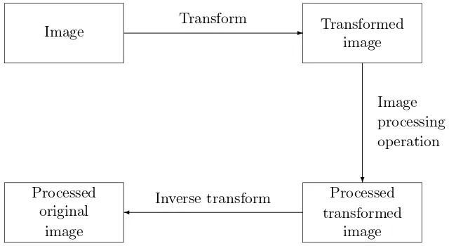
1. Transforms. A “transform” represents the pixel values in some other, but equivalent form. Transforms allow for some very efficient and powerful algorithms, as we shall see later on. We may consider that in using a transform, the entire image is processed as a single large block. This may be illustrated by the diagram shown in figure 2.1.
✁
Image Transformed
image
Processed transformed
image Processed
original image
Transform
Inverse transform
[image:41.595.154.474.392.567.2]Image processing operation
Figure 2.1: Schema for transform processing
2. Neighbourhood processing. To change the grey level of a given pixel we need only know the value of the grey levels in a small neighbourhood of pixels around the given pixel.
3. Point operations. A pixel’s grey value is changed without any knowledge of its surrounds. Although point operations are the simplest, they contain some of the most powerful and widely used of all image processing operations. They are especially useful in image pre-processing, where an image is required to be modified before the main job is attempted.
2.2
Arithmetic operations
These operations act by applying a simple function ✂✁ ✠☞☛ ✌
to each grey value in the image. Thus ✠☞☛ ✌
is a function which maps the range✥ ✕ ✕ ✕
✜☛✜
onto itself. Simple functions include adding or subtract a constant value to each pixel:
✂✁ ☛✁✄✂
or multiplying each pixel by a constant: ✂✁☎✂ ☛ ✕
In each case we may have to fiddle the output slightly in order to ensure that the results are integers in the✥
✕ ✕ ✕ ✜☛✜
range. We can do this by first rounding the result (if necessary) to obtain an integer, and then “clipping” the values by setting:
✝✆
✞
✜☛✜
if ✠✟ ✜☛✜
,
✥
if ✁ ✥ .
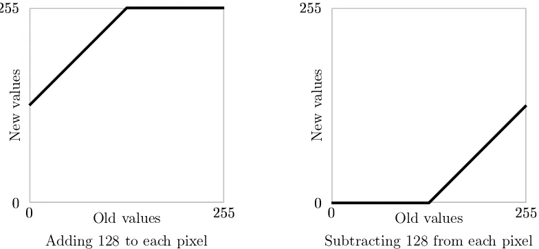
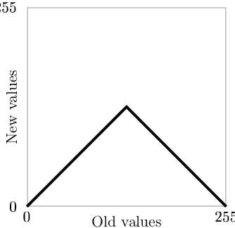
We can obtain an understanding of how these operations affect an image by plotting ✁ ✠☞☛ ✌ . Figure 2.2 shows the result of adding or subtracting 128 from each pixel in the image. Notice that
✥
✥
✜☛✜ ✜☛✜
Old values
N
ew
va
lu
es
Adding 128 to each pixel
✥
✥
✜☛✜ ✜☛✜
Old values
N
ew
va
lu
es
[image:42.595.111.503.345.526.2]Subtracting 128 from each pixel
Figure 2.2: Adding and subtracting a constant
when we add 128, all grey values of 127 or greater will be mapped to 255. And when we subtract 128, all grey values of 128 or less will be mapped to 0. By looking at these graphs, we observe that in general adding a constant will lighten an image, and subtracting a constant will darken it.
We can test this on the “blocks” image blocks.tif, which we have seen in figure 1.4. We start by reading the image in:
>> b=imread(’blocks.tif’); >> whos b
Name Size Bytes Class
The point of the second command was to find the numeric data type of b; it isuint8. The unit8 data type is used for datastorage only; we can’t perform arithmetic operations. If we try, we just get an error message:
>> b1=b+128
??? Error using ==> +
Function ’+’ not defined for variables of class ’uint8’.
We can get round this in two ways. We can first turn binto a matrix of type double, add the 128, and then turn back touint8 for display:
>> b1=uint8(double(b)+128);
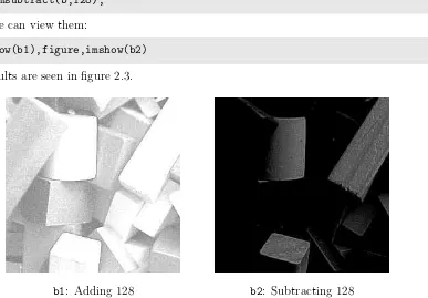
A second, and more elegant way, is to use theMatlab function imadd which is designed precisely to do this:
>> b1=imadd(b,128);
Subtraction is similar; we can transform out matrix in and out of double, or use the imsubtract function:
>> b2=imsubtract(b,128);
And now we can view them:
>> imshow(b1),figure,imshow(b2)
and the results are seen in figure 2.3.
[image:43.595.127.514.334.603.2]b1: Adding 128 b2: Subtracting 128
Figure 2.3: Arithmetic operations on an image: adding or subtracting a constant
✥
✥
✜☛✜ ✜☛✜
Old values
N
ew
va
lu
es
✁ ☛✁
✥
✥
✜☛✜ ✜☛✜
Old values
N
ew
va
lu
es
✁ ☛
✥
✥
✜☛✜ ✜☛✜
Old values
N
ew
va
lu
es
✂✁ ☛✂ ✎
✏
✢
Figure 2.4: Using multiplication and division
✂✁ ☛✁
b3=immultiply(b,0.5); orb3=imdivide(b,2) ✂✁ ☛
b4=immultiply(b,2);
✂✁ ☛✁ ✎
✏
✢
b5=imadd(immultiply(b,0.5),128);or b5=imadd(imdivide(b,2),128);
Table 2.1: Implementing pixel multiplication byMatlabcommands
b3: ✁ ☛✂
b4: ✁ ☛
b5: ✂✁ ☛✂ ✎
✏
✢
still quite clear, whereas a lot of information has been lost by the subtraction process, as can be seen in image b2. This is because in image b2 all pixels with grey values 128 or less have become zero.
A similar loss of information has occurred in the images b1 and b4. Note in particular the edges of the light coloured block in the bottom centre; in both b1and b4 the right hand edge has disappeared. However, the edge is quite visible in imageb5.
Complements
The complement of a greyscale image is its photographic negative. If an image matrixm is of type double and so its grey values are in the range ✥
✕
✥
to ✏
✕
✥
, we can obtain its negative with the command
>> 1-m
If the image is binary, we can use >> ~m
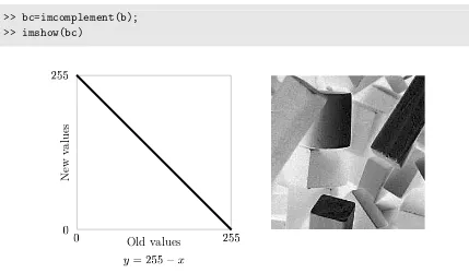
If the image is of type uint8, the best approach is the imcomplement function. Figure 2.6 shows the complement function ✂✁
✜☛✜
☛
, and the result of the commands >> bc=imcomplement(b);
>> imshow(bc)
✥
✥
✜☛✜ ✜☛✜
Old values
N
ew
va
lu
es
✂✁ ✜☛✜
☛
Figure 2.6: Image complementation
[image:45.595.83.512.374.624.2]✥
✥
✜☛✜ ✜☛✜
Old values
N
ew
va
lu
es
Complementing only dark pixels
✥
✥
✜☛✜ ✜☛✜
Old values
N
ew
va
lu
es
[image:46.595.333.500.67.229.2]Complementing only light pixels
Figure 2.7: Part complementation
2.3
Histograms
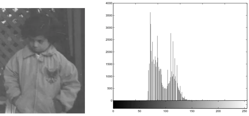
Given a greyscale image, its histogram consists of the histogram of its grey levels; that is, a graph indicating the number of times each grey level occurs in the image. We can infer a great deal about the appearance of an image from its histogram, as the following examples indicate:
In a dark image, the grey levels (and hence the histogram) would be clustered at the lower end:
In a uniformly bright image, the grey levels would be clustered at the upper end:
In a well contrasted image, the grey levels would be well spread out over much of the range: We can view the histogram of an image inMatlab by using theimhistfunction:
>> p=imread(’pout.tif’);
>> imshow(p),figure,imhist(p),axis tight
(theaxis tight command ensures the axes of the histogram are automatically scaled to fit all the values in). The result is shown in figure 2.8. Since the grey values are all clustered together in the centre of the histogram, we would expect the image to be poorly contrasted, as indeed it is.
Given a poorly contrasted image, we would like to enhance its contrast, by spreading out its histogram. There are two ways of doing this.
2.3.1 Histogram stretching (Contrast stretching)
Suppose we have an image with the histogram shown in figure 2.9, associated with a table of the numbers ✂✁ of grey values:
Grey level ✄ ✥
✏
✒ ✛ ✜ ✪ ✭ ✢ ☎
✏
✥
✏ ✏ ✏ ✏
✒
✏
✛
✏
✜
✆✁
✜ ✥ ✥ ✥ ✥ ✭ ✥ ✥
✛
0 50 100 150 200 250 0
[image:47.595.101.516.119.313.2]500 1000 1500 2000 2500 3000 3500 4000
Figure 2.8: The imagepout.tifand its histogram
✔✁
✌
✁
✂✔✁ ✑✔✁ ✂✁✔✁ ✁✔✁
✁ ✗ ✌ ✕ ✂
✧
✑✁ ✂✁ ✔ ✁ ✂✗ ✌ ✂✕
✁
✗
✌
✕
✂
✧
✑
✂✁ ✔ ✁ ✂✗
✌
✂✕
✁ ✗ ✌ ✕ ✂
✧
✑✂ ✂✁ ✔ ✁ ✂✗ ✌ ✂✕
(with ✁ ✒ ✪ ✥
, as before.) We can stretch the grey levels in the centre of the range out by applying the piecewise linear function shown at the right in figure 2.9. This function has the effect of stretching the grey levels ✜
–☎
to grey levels –✏ ✛
according to the equation: ✁ ✏
✛
☎ ✜
✠
✄ ✜ ✌✡✎
where ✄
is the original grey level and its result after the transformation. Grey levels outside this range are either left alone (as in this case) or transformed according to the linear functions at the ends of the graph above. This yields:
✄ ✜ ✪ ✭ ✢ ☎
✜ ✢
✏ ✏ ✏
✛
and the corresponding histogram:
✔✁
✌
✁
✂✔✁ ✑✔✁ ✂✁✔✁ ✁✔✁
✁ ✗
✌
✕ ✂
✧
✑ ✂✁ ✔ ✁ ✂✗
✌
✂✕
which indicates an image with greater contrast than the original. Use of imadjust
To perform histogram stretching in Matlab the imadjust function may be used. In its simplest incarnation, the command
imadjust(im,[a,b],[c,d])
stretches the image according to the function shown in figure 2.10. Since imadjustis designed to
✁ ✂
✏
✄
[image:48.595.209.399.258.416.2]✏
work equally well on images of type double, uint8 or uint16 the values of ✁ , ✂
, and ✄
must be between 0 and 1; the function automatically converts the image (if needed) to be of typedouble.
Note that imadjust does not work quite in the same way as shown in figure 2.9. Pixel values less than ✁
are all converted to , and pixel values greater than ✂
are all converted to✄
. If either of [a,b] or [c,d] are chosen to be [0,1], the abbreviation []may be used. Thus, for example, the command
>> imadjust(im,[],[])
does nothing, and the command >> imadjust(im,[],[1,0])
inverts the grey values of the image, to produce a result similar to a photographic negative. The imadjust function has one other optional parameter: the gamma value, which describes the shape of the function between the coordinates ✠ ✁ ✁ ✌
and ✠
✂
✁
✄
✌
. If gammais equal to 1, which is the default, then a linear mapping is used, as shown above in figure 2.10. However, values less than one produce a function which is concave downward, as shown on the left in figure 2.11, and values greater than one produce a figure which is concave upward, as shown on the right in figure 2.11.
✁
✂
✏
✄
✏
gamma ✁
✏
✁
✂
✏
✄
✏
gamma ✟
✏
Figure 2.11: Theimadjustfunction with gammanot equal to 1
The function used is a slight variation on the standard line between two points: ✂✁
✁
☛ ✁
✂
✁✄✂✆☎
✠
✄
✌✡✎ ✕
Use of the gamma value alone can be enough to substantially change the appearance of the image. For example:
>> t=imread(’tire.tif’); >> th=imadjust(t,[],[],0.5); >> imshow(t),figure,imshow(th)
produces the result shown in figure 2.12.
We may view the imadjuststretching function with the plotfunction. For example, >> plot(t,th,’.’),axis tight
Figure 2.12: The tire image and after adjustment with thegammavalue
0 50 100 150 200 250
0 50 100 150 200 250
[image:50.595.187.423.430.632.2]A piecewise linear stretching function
We can easily write our own function to perform piecewise linear stretching as shown in figure 2.14. To do this, we will make use of the findfunction, to find the pixel values in the image between ✁
✁
and ✁
✁✁ . Since the line between the coordinates ✠✁ ✁ ✁ ✂ ✁ ✌
and ✠✁ ✁✂
✁
✂
✁✁
✌
has the equation
[image:51.595.251.368.140.257.2]✁ ✁ ✁ ✗ ✁ ✌ ✂ ✂ ✂ ✗ ✂ ✌
Figure 2.14: A piecewise linear stretching function
✂✁ ✂ ✁✁ ✂ ✁ ✁ ✁✁ ✁ ✁ ✠☞☛ ✁ ✁ ✌ ✎ ✂ ✁
the heart of our function will be the lines pix=find(im >= a(i) & im < a(i+1));
out(pix)=(im(pix)-a(i))*(b(i+1)-b(i))/(a(i+1)-a(i))+b(i);
whereimis the input image andoutis the output image. A simple procedure which takes as inputs images of typeuint8 or doubleis shown in figure 2.15. As an example of the use of this function:
>> th=histpwl(t,[0 .25 .5 .75 1],[0 .75 .25 .5 1]); >> imshow(th)
>> figure,plot(t,th,’.’),axis tight
produces the figures shown in figure 2.16.
2.3.2 Histogram equalization
The trouble with any of the above methods of histogram stretching is that they require user input. Sometimes a better approach is provided by histogram equalization, which is an entirely automatic procedure. The idea is to change the histogram to one which is uniform; that is that every bar on the histogram is of the same height, or in other words that each grey level in the image occurs with the saem frequency. In practice this is generally not possible, although as we shall see the result of histogram equalization provides very good results.
Suppose our image has ✄
different grey levels ✥
✁
✏
✁ ✁ ✕ ✕ ✕
✄
✏ , and that grey level
✄
occurs ✁ times in the image. Suppose also that the total number of pixels in the image is (so that
✁
✎ ✎ ✎✆☎✝☎✝☎ ✎ ✟✞
✦
✁
. To transform the grey levels to obtain a better contrasted image, we change grey level✄
to ✁ ✁ ✎ ✎✠☎✝☎✝☎ ✎ ✁ ✂ ✠ ✄ ✏ ✌✖✕
function out = histpwl(im,a,b) %
% HISTPWL(IM,A,B) applies a piecewise linear transformation to the pixel values % of image IM, where A and B are vectors containing the x and y coordinates % of the ends of the line segments. IM can be of type UINT8 or DOUBLE, % and the values in A and B must be between 0 and 1.
%
% For example: %
% histpwl(x,[0,1],[1,0]) %
% simply inverts the pixel values. %
classChanged = 0; if ~isa(im, ’double’),
classChanged = 1; im = im2double(im); end
if length(a) ~= length (b)
error(’Vectors A and B must be of equal size’); end
N=length(a);
out=zeros(size(im));
for i=1:N-1
pix=find(im>=a(i) & im<a(i+1));
out(pix)=(im(pix)-a(i))*(b(i+1)-b(i))/(a(i+1)-a(i))+b(i); end
pix=find(im==a(N)); out(pix)=b(N);
if classChanged==1 out = uint8(255*out); end
0 50