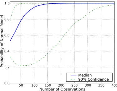
IV.5 Posterior probability for the normal model (candidate models are the . normal and lognormal) as a function of sample size. Using this optimization, a quality surrogate model can be constructed at a small fraction of the cost typically required by other response surface methods.
Reliability Analysis
- Mean Value Method
- MPP-Based Methods
- Sampling Methods
- Hybrid Methods
- Surrogate Models
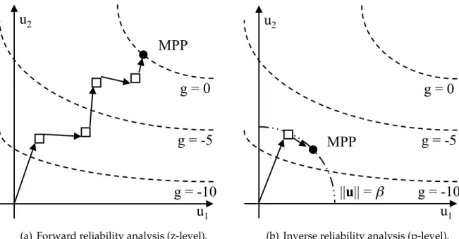
The value of the response function at the optimal MPP solution G(u∗) determines the desired output of the response level. AMV in u-space: A single linearization of the response function performed in u-space on the mean values of the input random variables.
Reliability-Based Design Optimization
Nested RBDO
The ability to provide this type of sensitivity information is an advantage of MPP-based methods, but due to the potential inaccuracy in these types of reliability analyses, they can lead to optimal solutions that do not satisfy the likelihood constraint. of failure. For Monte Carlo sampling, estimated sensitivities can be derived, but in a nested formulation the probability of failure may need to be calculated a large number of times (depending on the number of iterations for optimization convergence), making Monte Carlo sampling rarely feasible. for RBDO because of the computational costs involved.
Single-Loop RBDO
The third constraint is the KKT optimality condition, the derivation of which (as described above) also relies on the assumption of the first-order boundary condition. However, the accuracy of the final solution relies on the accuracy of the underlying first-order assumption.
Sequential RBDO
Sequential RBDO is more efficient than the nested formulation, but generally more expensive than the single-loop formulation. It can be more accurate than single-loop results due to the possible inclusion of higher-order approximations to the limit state, but will still be inaccurate if these approximations are poor.
Summary
Engineers are then forced to revert to sampling methods that do not rely on MPP convergence or simplifying approximations to the true shape of the limit state. This chapter develops a method based on efficient global optimization47 (EGO) to adaptively search for multiple points at or near the limit state throughout the space of random variables.
Efficient Global Optimization
Gaussian Process Models
This variance indicates uncertainty in the GP model arising from the construction of the covariance function. This form of variance takes into account the uncertainty of the trend β coefficients, but assumes that the parameters governing the covariance function (σZ2 and θ) have known values.
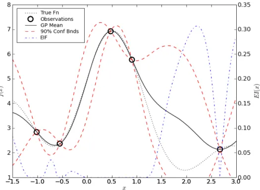
Expected Improvement Function
Because the magnitude of the EIF peak is used as the convergence criterion, this may cause problems in evaluating the convergence of EGO. Instead of basing the convergence on the EIF as shown, it is first scaled by the absolute value of the constant term from the trend of the underlying GP model, i.e.
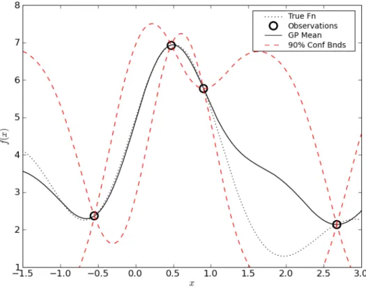
Simple EGO Example
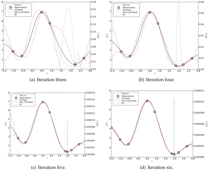
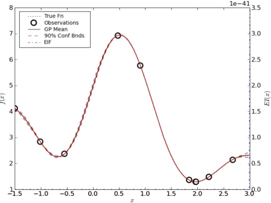
This completes the first iteration of the EGO algorithm and the new state of knowledge is shown in Figure II.5. Note that with each iteration, the value of the EIF at the maximization point (shown on the scale to the right of each graph) is decreased in each iteration.
Expected Feasibility Function
In this case, maximizing EIF is inappropriate because the main concern is feasibility. Like EIF, the magnitude of EFF will be affected by the magnitude of the underlying response function g(x).
Efficient Global Reliability Analysis Algorithm
Because all MAIS samples are evaluated using the GP model, they can be provided at low cost. While EGO/EGRA will typically need far fewer evaluations of the true objective/response function than other methods, they both require a non-trivial amount of computational overhead to construct the GP models and to solve the global optimization problem to maximize the EIF/ EFF.
Computational Experiments
Multimodal Function
Most MPP search methods converge to the same MPP and thus report the same probability. This shows that the GP model produced by EGRA is an extremely accurate representation of the true function.
Cubic Function
EGRA and LHS: the error in the mean probability and the mean of the absolute errors from 20 independent simulations. Again, second-order integration produces better results, but is still not an accurate approximation of the true form of the limit state, so there are still large errors.
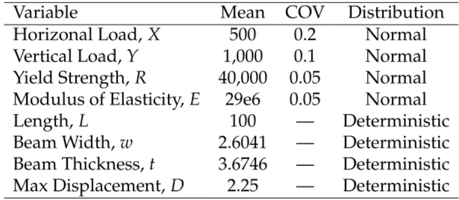
Cantilever Beam
To create an accurate estimate of the true solution, 20 independent simulations were run using one million Latin hypercube samples per simulation. Again, two errors are reported for EGRA and LHS: the error in the mean probability and the mean of the absolute errors from 20 independent simulations.
Short Column
EGRA required only one-third the number of feature evaluations of the least expensive MPP-based method, but again produced an accuracy comparable to exhaustive LHS. The accuracy of the EGRA results is comparable to using 100,000 LHS samples, but clearly comes at a much reduced cost.
Steel Column
To establish an accurate estimate of the true solution, 20 independent studies were performed with one million Latin hypercube samples per examination. Again, two errors are reported for EGRA and LHS: the error in the mean probability and the mean of the absolute errors from the 20 studies.
Bistable MEMS Device
The manufactured thickness of the device is also variable, although this does not contribute as much to the variability in the force-displacement behavior. A remarkable feature of these results is that EGRA requires less than one-third the number of function evaluations than cheaper MPP search methods, and the average error in EGRA solutions is significantly smaller than for LHS solutions.

Summary
The cost of EGRA is driven by three factors: the size of the search space, the shape of the response function, and the probability of failure. If the probability of failure is low, then the size of the failure region relative to the search space is small.
Previous Methods
In general, any of the previously discussed methods can be used to locate the MPP for each of the components. With these in place, let represent the vector of reliability indices for each of the components, and let represent the correlation matrix between the failure modes of the components (calculated as dot products of -∇k∇uGiT . uGik).
Formulations Using EGRA
Component Solutions
Because EGRA has already been shown to be an efficient and accurate method for constructing surrogate models of the component limit states, it will similarly provide an efficient and accurate method for solving the system-level problem. The following two methods provide ways in which EGRA can focus its efforts only on the limit conditions that bound the failure region of the system.
Composite Gaussian Process Model
EGRA can be encouraged to search for this composite limit state by a simple modification of the response function. The second problem with fitting a composite GP model is the presence of the sharp corners in the composite limit state.
Composite Expected Feasibility Function
Once this point is found, the EFF value for each of the components is calculated at that point. The results of this method are explored in more detail in the discussion of the first computational experiment presented in the next section.
Computational Experiments
Multimodal System
This does not affect the shape of the composite limit state or the behavior of the EGRA. Similar to the result for the parallel system, EGRA focuses the training data only near the limit state portions of the components that form the composite limit state (i.e., limit the failure region of the system).
Cantilever Beam
Liquid Hydrogen Tank
To obtain an accurate estimate of the actual solution, twenty independent simulations were performed using one million Latin hypercube samples per simulation. To measure the accuracy of the method, two errors are reported for the EGRA results: the error in the mean probability and the average of the absolute errors from twenty independent simulations.
Summary
Consequently, there is also a certain amount of uncertainty associated with any estimate of probability of failure calculated with a reliability analysis based on the assumed probability distribution models. Uncertainty associated with a probability distribution model can be divided into two parts: uncertainty about the probability distribution model form and uncertainty about the model parameters.
Bayesian Inference and Model Averaging
Bayesian Inference
R π(θ)p(d| θ)dθ, (IV.2) where p(θ|d) is the posterior distribution for θ, π(θ) is the so-called prior distribution and p(d|θ) is the probability function for θ. However, Markov Chain Monte Carlo (MCMC) sampling has been shown to be an effective method for simulating (by random sampling) the posterior distribution.
Bayesian Model Averaging
Adding the uncertainty of the model shape, it is easy to show that the posterior distribution of γ is given by . The posterior distribution of the quantity of interest, γ, is then a comprehensive representation of the uncertainty associated with γ due to uncertainty in both the shape of the probability distribution model and the parameters associated with the input random variable.
Reliability Analysis Under Uncertainty
Generate a random realization of the probability density function p(x):. a) Randomly select a probability distribution model Mj based on the model form posterior probabilities,P(Mr |d),r =1,. The results of this sampling scheme can be used to derive a variety of metrics that are useful in conveying the impact of probability distribution model uncertainty on the results of the reliability analysis.
Computational Experiments
Cantilever Beam with Parameter Uncertainty
The end result is the posterior distribution of the failure probability for each response function, as shown in Figure IV.1. These graphs show a clear convergence of the posterior distributions towards the true failure probability.
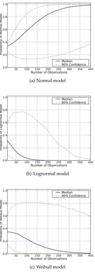
Convergence of Model Form with Additional Data
For the normal model, it can be shown that the parameters ˆθ = (µ, ˆˆ σ) maximize the likelihood function (and also the log-likelihood function). Unlike the normal and lognormal distributions, maximum likelihood estimation of the Weibull parameters is not available in closed form.
Bistable MEMS
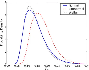
The previous analysis is repeated with the addition of the Weibull model as a possible form of probability distribution model. The resulting posterior distribution (based on 5000 analyses) of pf is shown in Figure IV.8, which shows a normalized histogram of 5000 pf samples together with a kernel72 density estimate based on these samples.
Summary
The approach is based on repeating the reliability analysis hundreds or thousands of times using feasible realizations of the input probability density functions suggested by the Bayesian inference. The first is to reduce the cost of performing the reliability analysis on a candidate design by reducing the number of evaluations of the response function required.
Constraint Formulations for EGO
Augmented Lagrangian Formulation
Note that this equation assumes the presence of only one of each type of constraint, but λg, λh, ∆g, and ∆h can easily be replaced by vectors to form a more general formulation. Recall that at any time, the terms ˆf, ˆ∆g, and ˆ∆h do not represent single values, but Gaussian distributions.
Expected Violation Function
In this study, the nonlinear interior point solver (NIPS) in OPT++59 is used to perform this solution improvement. Additional details on the implementation of the merit function can be found in Ref.
Simple Constrained EGO Example
EGO clearly does a good job of enforcing the restriction; none of the solutions were impossible. EGO is also less expensive than NIPS, requiring only 61% of the total feature evaluations (on average).
Formulations for RBDO with EGO/EGRA
Nested RBDO with Separate Surrogates
This successful test shows that this constrained EGO method promises to solve the RBDO problem, which also includes a nonlinear inequality constraint.
Nested RBDO with a Single Surrogate
However, the disadvantage of this method is that it can "ruin" function evaluations by solving the boundary condition in regions of the design space that can never be visited by the optimizer. For the tests of this method in Section V.3, a full EGRA analysis is performed using the true response function to verify the reliability of the optimal design.
Sequential RBDO
Instead, this study uses a metric on the accuracy of the underlying GP constraint function models. At the optimal point from an EGO solution, if the value of all GP models of the constraint functions is within 1% of the actual values of the constraint function after verification, the method is said to have converged.
Computational Experiments
- Short Column
- Cantilever Beam
- Liquid Hydrogen Tank
- Steel Column
- Bistable MEMS
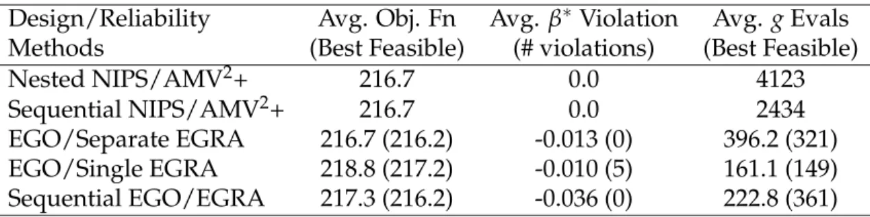
It used approximately 16% of the function ratings required by the NIPS/AMV2+ follow-up baseline test. The final RBDO test involves the design of the bistable MEMS device presented in Section II.4.6.
Summary
This new surrogate model is then used in place of the true function in a sampling method. Obviously, the location of the limit state contour in random variable space cannot do that.
Future Work
Extensions to EGRA
A parallel implementation of EGO and EGRA will locate all the local optima at each iteration. The next extension will enable EGRA to solve for multiple response levels to solve for the full CDF of the response rather than the probability of failure at a single response level.
Additional Applications of EGRA
An important feature of EGRA is how it minimizes the error of the surrogate model by using a measure of convergence that is based in part on the variance of the GP. Quantifying the impact of Gaussian process model error on the reported failure probability is not entirely straightforward, but should not require any changes to the EGRA algorithm itself.
Improvements to EGO and EGRA
If the EGO converged on the boundaries of space, the confidence region would be translated and/or expanded. However, the accuracy of the boundary condition in this region is relatively unimportant because the probability of events in this region is so small.
Expected Improvement Function
In the integral in the first term above, introduce the change of variablekw=v22, which gives dv=1vdw.
Expected Feasibility Function
Expected Violation Function for Equality Constraints
- Results for the multimodal problem
- Results for the cubic function problem
- Results for the stress function of the cantilever beam problem
- Results for the displacement function of the cantilever beam problem
- Results for short column problem
- Results for the steel column test problem
- Results for the bistable mems device problem
- Results for the parallel multimodal system problem
- Results for the series multimodal system problem
- Results for the cantilever beam system problem
- Results for the liquid hydrogen tank system problem
- Variable detail for the cantilever beam example. The values for t, w, and
- Model form posterior probabilities based on 20 observations of ∆W
- Results for the simple constrained EGO example
- Results for the short column RBDO example
- Variable detail for the cantilever beam example
- Results for the cantilever beam RBDO example
- Results for the liquid hydrogen tank RBDO problem
- Results for the steel column RBDO example
- Results for the bistable MEMS RBDO example
- Possible reliability analysis iteration histories
- Comparison of (a) basic Monte Carlo and (b) Latin Hypercube sampling. 11
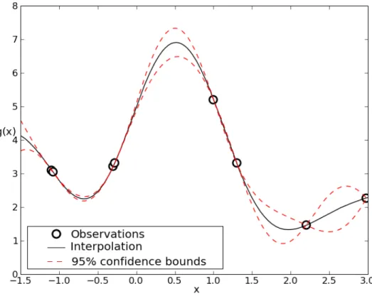
- Plot of simple Gaussian process model
- Simple EGO example - True function to be minimized
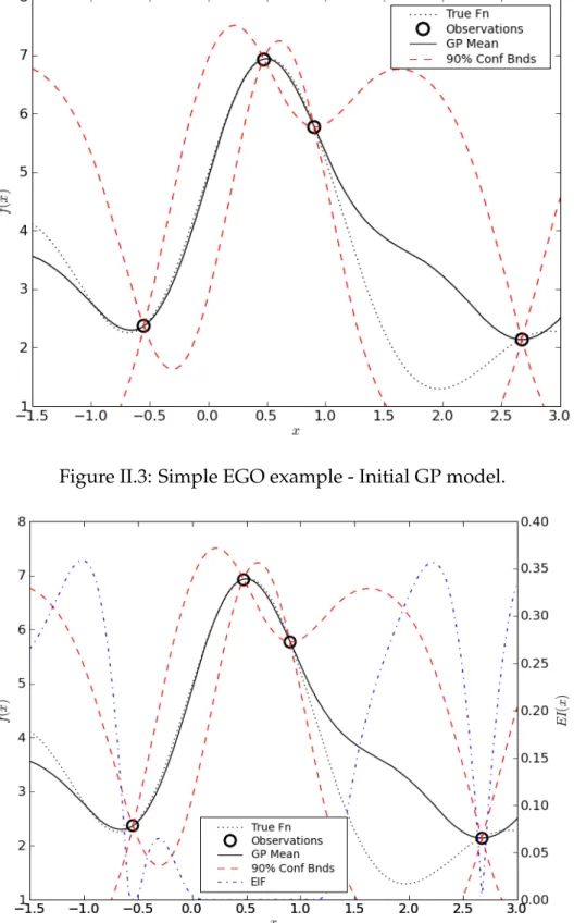
- Simple EGO example - Initial GP model
- Simple EGO example - Initial EIF
- Simple EGO example - Iteration two
- Simple EGO example - Iterations 3-6
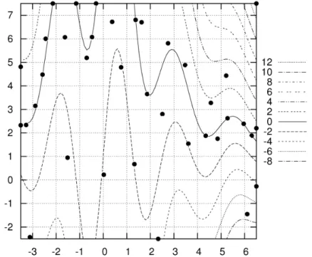
- Simple EGO example - Final iteration
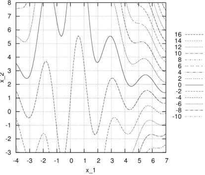
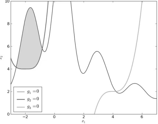
- Contour plot of the multimodal function. The solid line is g = z ¯ = 0
- Contours of the mean value (solid line is the limit state), variance, and
- Contours of the mean value (solid line is the limit state), variance, and
- Contours of the mean value (solid line is the limit state), variance, and
- Contours of the mean value (solid line is the limit state), variance, and
- Final contour of the mean value (solid line is the limit state) with 37
- Schematic of the cantilever beam example problem
- Bi-stable MEMS mechanism
- Tapered beams for bistable MEMS mechanism
- Contour plot of F min ( d, x ) as a function of uncertain variables x. Solid
- Graphical depiction of the composite limit state. The lines are compo-
- Results from running EGRA on the composite response function. Note
- Limit state contours of the multimodal system response functions. The
- Resulting GP models and training data from a run of EGRA on the par-
74] Sirimamilla, R., Venkataraman, S., and Pai, S., Integrating data uncertainty into reliability-based design optimization using inverse reliability measures, Proc. 78] Tu, J., Choi, K.K., and Park, Y.H., A New Study on Reliability-Based Design Optimization, Journal of Mechanical Design, Vol.