INFORMATION QUANTITIY AND ORDER IN STUDENTS’ TAX RESEARCH JUDGMENTS
Alexander M.G. Gelardi Associate Professor University of St. Thomas1
Received: April 11 2009 Accepted: June 30, 2010
Abstract
The Belief Adjustment model predicts recency effects for complex information encoded in a step-by-step process. However, the literature indicates that the recency effect may not carry-over to larger numbers of pieces of information. This may be a problem with the amount of information now available through the internet.
Tax research tasks can have a number of pieces of information (cues). How tax students process information has not been studied extensively. This study extended prior work by investigating the effect of series of four, eight, and twelve cues on tax decisions made by undergraduate tax students.
It was found that there was a strong overall recency order effect. However, the recency order effect seemed to be driven by the longer cue series, rather than by the shorter cue series. This is contrary to the predictions of the Belief Adjustment model.
Keywords:
Accounting Recency Tax Judgments Belief Adjustment ModelJEL Classifications: H24, H29, H34, C12, C21, C91, M41
1 Opus College of Business, University of St. Thomas, 1000 LaSalle Avenue, TMH#443 Minneapolis, MN, 55403-4710 Phone: 651-962-4402 Fax: 651-962-4710
Email: [email protected]
1. Introduction
Students are required to carry out some research task in many of their tax courses. They research some area of tax law and make a judgement based on the findings. Several different sources of authority may be consulted: tax services and electronic data bases may be used. Searches on the internet have expanded ability to find potential sources of information. The amount of information available can be extremely large. Information from these media sources is, by necessity, obtained sequentially and can contain conflicting messages.
Prior studies have found that the order in which information is presented and processed can affect judgments in sequential information processing tasks (see Hogarth and Einhorn 1992 for a review).
However, some uncertainty exists whether this order effect can be generalized to legal tax research contexts. Studies using experiments in accounting contexts to examine order effects may not typify tax decision making because these studies tended to use balanced information sets of two or four pieces of information (cues) in the experimental tasks.
To prepare students to carry out legal tax research in practice, the students are often presented with more than four pieces of information. This is designed to correspond to a typical legal tax research task, where a tax advisor is likely to obtain a number of pieces of information, as well as to consult different sources of authority.
This study extends prior research by examining order effects in tax research decisions of students.
The experiment tested for order effects in tax judgments using information sets of four, eight and twelve pieces of information.
The results of this study show that order effects do exist in a legal tax research setting, especially where the number of pieces of information is large. This would indicate that there is the possibility that tax judgments are systemically biased. Therefore, the tax research tasks should be designed so that information is given in a mixed order, as opposed to a more "helpful" order. Also, students should be trained not to group the results of their research, using tax authorities (cases, revenue rulings etc.), into lists that support a certain position and that do not support that position (to carry out more detailed research with those authorities).
The rest of this paper is organized in the following manner. The next section briefly outlines some theoretical aspects of belief revision in decision making. Prior empirical studies using the model in accounting contexts are outlined. The hypotheses tested in this study are then specified in the following section. The experiments conducted are described. The data analysis and the experimental results are presented. A discussion of the findings and the limitations of the study precede the summary section.
2. Theoretical Framework
Several authors have found that human beings do not follow the Bayesian model when adjusting their beliefs but are influenced by normatively irrelevant factors (e.g., Kahneman and Tversky, 1972, 1979;
Hogarth, 1987; Markowitz, 1952]. One such factor that has been empirically observed is an order effect.
That is, the order in which information is received by the decision maker can affect the decision made (see Hogarth and Einhorn, 1992 for an extensive review). This paper uses the Belief Adjustment model (Hogarth and Einhorn, 1992) as its theoretical base.
In the Belief Adjustment model, Hogarth and Einhorn (1992) examine the effects of evidence on a decision maker's revision of his belief. They consider some task variables predicted to have an effect on the outcomes. Specifically, they consider the complexity of the actual subject matter, the number of
information cues that have to be considered, the encoding reference background and the response mode used to elicit the judgments. Two types of response modes are considered. One is whether the belief is adjusted after each piece of evidence is received (step by step ["SbS"]). The other is whether belief is adjusted after looking at all the pieces of evidence (end of sequence ["EoS"]). The encoding reference backgrounds are either the hypothesis being considered ("evaluation") or the current anchor ("estimation").
The Belief Adjustment Model
The model is based on the premise that persons formulate an opinion on the first piece of evidence they see (or, alternatively, have a prior belief) and then adjust from this belief with any new evidence obtained. In effect, this is the sequential anchor-and-adjustment strategy specified by Tversky and Kahneman (1974).
The model also looks at processes involved where only one decision is being made. The model is not intended to cover situations in which several decisions or hypotheses are interdependent [cf., Robinson and Hastie, 1985]. Further, this model is concerned with the updating of a hypothesis, not the construction of a hypothesis over time. Construction of a hypothesis, as in the Pennington and Hastie (1986) experiments, can give results not predicted by the Belief Adjustment model.
The basic form of the model is:
Sk = Sk-1 + Wk[S(Xk)-R] (1) where
Sk = Degree of belief in some hypothesis after evaluating k pieces of evidence (O ≤ Sk ≤ 1).
Sk-1 = Anchor or prior belief. Initial belief is So. Wk = An adjustment weight for the kth piece of evidence.
S(Xk) = Subjective evaluation of the kth piece of evidence.
R = Background reference point against which the impact of the kth piece of evidence is being evaluated.
The difference between the evaluation of the kth piece of evidence and some reference background is the representation of the encoding process. This is shown as [S(Xk)-R] in equation 1. Hogarth and Einhorn envisage two types of encoding modes and related backgrounds against which the kth piece of evidence is evaluated. These types of encoding modes can be labelled as evaluation or estimation. In the evaluation mode, the reference background is the hypothesis being considered. Evaluation involves deciding whether or not the hypothesis is true. The current belief can be expressed by some value on a continuum that the hypothesis is true or false. In this case, evidence that supports the hypothesis always increases one's belief in the hypothesis, whereas disconfirming evidence always decreases the belief.
Thus, the evidence is seen as being bipolar. The background reference point is stable. The evidence is considered to be positive or negative with respect to the hypothesis, thus it gives -1 ≤ S(Xk) ≤ 1 and R=0.
Substituting R=0 in equation 1 gives
Sk = Sk-1 + WkS(Xk). (2) In the estimation mode, the background against which the new piece of evidence is evaluated is the
belief held at that time, the current anchor. If the strength of the new piece of evidence is greater than the anchor, the belief will increase. If the strength of the new piece of evidence is less than that of the current anchor, the belief will decrease. The same piece of evidence can be regarded as positive or negative depending on the current belief. Thus, the evidence can be seen as being unipolar. The background reference point is dynamic. The evidence is considered to be positive or negative with respect to the current belief, giving 0 ≤ S(Xk) ≤ 1 and R=Sk-1. Substituting R=Sk-1 in equation 1 gives
Sk = Sk-1 + Wk[S(Xk)-Sk-1]. (3) Rearranging the terms, equation 3 becomes
Sk = (1-Wk)Sk-1 + WkS(Xk). (4) This is the averaging form of the model.
The evaluation mode with the stable background is similar to Anderson's (1981) additive model; the estimation mode with the dynamic background is similar to Anderson's averaging model. Hogarth and Einhorn (1992) give a further illustration of the difference between the evaluation and the estimation encoding modes. Suppose that one is required to update a neutral belief and that two pieces of evidence are received sequentially. Also, suppose that these items are both positive, although one is weak and the other is strong. If assessed on a bipolar evaluation scale, the evidence may have values of +0.8 and +0.2.
If assessed on a unipolar estimation scale both pieces of evidence would have values of greater than 0.5, say 0.9 and 0.6, under the assumption that the current belief is 0.5 (i.e., neutrality on the unipolar scale).
In the evaluation mode, both pieces of evidence would increase the belief because they are both encoded as positive. It does not matter in which order the pieces of evidence are received. However, the encoding process is different in the estimation mode. If the pieces of evidence were received in a weak-strong order, then, because 0.6 is greater than 0.5 and 0.9 is greater than the average of 0.6 and 0.5, both pieces of evidence would result in an upward belief adjustment. If the evidence were received in a strong-weak order, the strong piece of evidence would increase the belief because 0.9 is greater than 0.5;
however, the weak piece of evidence would decrease the belief because 0.6 is less than the average of 0.9 and 0.5.
To give a tax example, consider the case of whether an item of income should be regarded as capital or ordinary income. In the evaluation mode, one would classify any new evidence as supporting the capital treatment (positive) or not (negative). In the estimation mode, the new piece of evidence is evaluated with regard to the current anchor. If one holds a very strong opinion that the item is capital but the new evidence only weakly supports that view, the new piece of evidence would be encoded as negative.
After the evidence is encoded, it is processed. A series of pieces of evidence can be processed in several ways. The usual ways are a) "step by step" (SbS) and b) "end of sequence" (EoS). When a
person uses the SbS process, he updates or changes his prior belief with each piece of new evidence.
When a person uses an EoS process, he updates his prior belief only after he has seen all the evidence. At first sight, these are similar to the response modes. The main difference is that the processes are those that are actually used for decision-making strategies, whereas the response modes are the required methods for responding in the experimental situation. It is possible that, when one is required to use an EoS response mode, one in fact uses an SbS process and reports only the final updated belief. This may be the case when the evidence series is long or complex (Hogarth and Einhorn, 1992).
The model shows that new evidence has an adjustment weight, Wk. The adjustment weight has to be sensitive to the fact that the impact of the evidence (S(Xk)-R) is either negative or positive, and also to the level of the prior anchor, Sk-1. When the evidence is negative or neutral (i.e., S(Xk) ≤ R), then the weight, Wk, is proportional to the prior anchor. This indicates that if the prior belief is low, then evidence deemed negative can only reduce one's belief further by a small amount. Whereas, if the prior belief is high, then negative evidence can reduce that belief to a greater extent. Thus,
Wk = αSk-1 when S(Xk) ≤ R. (5A) The term α is the decision maker's sensitivity to negative evidence.
Where the new evidence is positive (i.e., S(Xk) > R), similar arguments to those above would indicate that the weight, Wk, is inversely proportional to the strength of the anchor. Thus,
Wk = β(1-Sk-1) when S(Xk) > R. (5B) The term β is the decision maker's sensitivity to positive evidence.
Different individuals may have different sensitivities to negative or positive evidence. A high (low) α indicates a high (low) sensitivity to negative evidence. Similarly, a high (low) β indicates a high (low) sensitivity to positive evidence. Thus, low α and β would indicate low sensitivity to new evidence, whereas high α and β show high sensitivity to new data. A skeptic would have a relatively high α and low β, and an advocate would have a relatively high β and low α. The relative strengths of α and β can dampen the order effects.
Step by step process. After each piece of evidence is received, the decision-maker updates his belief.
He then uses that new belief as the anchor for the adjustment he makes after observing the next piece of evidence. Thus, Equations 5A and 5B are placed into Equation 1 to obtain:
Sk = Sk-1 + αSk-1 [S(Xk)-R] when S(Xk) ≤ R. (6A)
Sk = Sk-1 + β[1-Sk-1][S(Xk)-R] when S(Xk) > R. (6B) The belief held after k pieces of evidence have been processed is a function of the following: a) the initial belief, b) the sequence in which the evidence was observed, c) the process by which the evidence was encoded, and d) the individuals' sensitivity to the direction of the evidence (positive or negative).
The sensitivity weights also indicate that the belief adjustment to new consistent evidence follows the
"Law of Diminishing Returns." That is, as more, say, positive evidence is received, the amount of belief
revision will be less and less. This concept follows from the proportionality of the adjustment weight, Wk, to the prior anchor.
End of sequence process. In the EoS process, the decision-maker updates his belief only after seeing all the evidence. There is only one belief change.
Sk = So + Wk [S(Xi,...,Xk)-R]. (7) S(Xi,...,Xk) is some function, possibly the weighted average, of the evaluations of each piece of evidence.
It is assumed that the scale value of the evidence does not vary with its position (i.e., first, third, etc.) in the sequential series.
The model is based on the premise that persons formulate an opinion on the first piece of evidence they see (or, alternatively, have a prior belief) and then adjust from this belief with any new evidence obtained. In effect, this is the sequential anchor-and-adjustment strategy specified by Tversky and Kahneman (1974).
This study examines a small subset of the model's predictions. It is considered that in a professional task the encoding reference background is evaluation and the response mode is SbS (Asare and Messier, 1991). Most tax research tasks are likely to be complex (as defined by Hogarth and Einhorn (1992) and may be either short or long.
Order Effect Predictions
The Belief Adjustment model makes a number of order effect predictions. The order effects depend on the type of processing used (SbS or EoS), the reference background (R=Sk-1 or R=0), the complexity of the task, and the length of the series of cues.
Under the SbS response mode, the model predicts a recency effect where R = Sk-1, in all cases.
When R=0, the model predicts no order effects where the evidence is consistent (all negative or positive).
If the evidence is mixed, then a recency effect is predicted, unless either α or β is approximately zero.
Where a negative piece of evidence is followed by a positive one (- +), the positive evidence is given more weight than if it had preceded the negative evidence. Similarly, where a negative item of evidence follows a positive one (+ -) the negative evidence is given more weight than if it had preceded the positive evidence. Thus, the recency effect gives a non-equivalence in the final belief. If the belief adjustments were graphed, then there would be a fish-tail effect (see Figure 1).
Figure 1
For a long series, the prediction is a primacy effect for consistent evidence in the evaluation encoding mode (R=0) and a force toward primacy for all other cases. Force toward primacy means that there is a recency effect that diminishes as the series becomes longer and eventually turns into a primacy effect.
Under the EoS response mode, the situation is more complex. If the task is simple, the model predicts a primacy effect, whether the encoding mode is evaluation or estimation, for both consistent and mixed evidence. Where the task is complex, the model makes several predictions: recency effects for both mixed and consistent evidence in the estimation mode, and for mixed evidence in the evaluation mode, but no order effect for consistent evidence in the evaluation mode.
Based on previous studies, Hogarth and Einhorn (1992) define a long series as twenty or more cues.
A short series is defined to be less than twelve cues. In most of those studies, the long series cues tended to be cognitively simple items such as adjectives. In all cases, there is a primacy or force toward primacy effect for long evidence series. This is similar to the concept of "attention decrement" set out by
Cues Belief
0 1 2
80
70
60
50
40
30
20
+- + -+
Fish Tail Effect
Anderson (1981).
Hogarth and Einhorn (1992) state that the reason for primacy is that persons may tire if they have to process too many items of evidence and also may become less sensitive to new information as the incremental value of that evidence is small. There may, however, be a third factor working in conjunction with these two. Although an anchoring and adjustment heuristic may be used, it is possible that where information is received over a short period of time, prior pieces of information can influence the decision.
If this is so, then the more pieces of information obtained the less influence some of the "middle" pieces of information will have (Murdock, 1962). Thus, the earlier pieces of information may have relatively greater influence, giving a force toward primacy.
Part of the complexity of predictions under the EoS response mode come about from the fact that the EoS response mode can elicit either EoS or SbS processing strategies. The SbS strategy is expected to be used where the task involves a long evidence series or is cognitively complex (Hogarth and Einhorn, 1992).
The model predicts recency for SbS response mode and primacy for EoS response mode, in short simple tasks. If the task is cognitively complex, then recency is predicted for mixed evidence in both response modes. There is a force toward primacy for long tasks in all cases.
In a tax context, it is suggested that the encoding mode will be evaluation, and so the background would be the hypothesis (i.e., R=0). This seems reasonable because most tax judgments tend to be on a dichotomous scale (cf., Asare and Messier, 1991). For example, one would have to decide whether or not a client is resident in country A for tax purposes, or whether a person is an employee or a self-employed contractor. The evidence in such judgments is bipolar.
Prior Experimental Evidence in Accounting
Prior research using the Belief Adjustment model in accounting has concentrated on using professionals, especially auditors, as subjects. The predictions of the model may be important in accounting decisions, as it is suggested that many judgments in accounting are formed from processing sequential information (Gibbins, 1984; Knechel and Messier, 1990).
Researchers using the Belief Adjustments model in a tax setting include Christian and Reneau (1989) who conducted four experiments using both undergraduate students and professional tax advisors. They examined both consistent evidence and mixed evidence. In the mixed evidence experiments, they found significant order effects for both the students and the tax professionals.
Christian and Reneau (1989), further, found that the tax professionals revised their beliefs by a greater amount for positive evidence than for negative evidence. The students revised their beliefs by approximately the same amount for both directions of the cues. This would suggest that tax professionals have higher sensitivity for positive evidence than for negative evidence (i.e. opposite results to those found with auditors) and consistent with the advocacy role.
This idea that tax professionals are more sensitive to positive pieces of information is supported by Johnson (1993), who found that tax professionals use a confirmatory process in belief adjustment. The assumption is that tax professionals initial belief supports that client’s view.
Ashton and Ashton (1988) examined an earlier version of the model in an auditing environment using professionals. They found results that were predicted by the model for both consistent evidence (no order effect) and mixed evidence (recency effect), under the SbS response mode. The authors also manipulated initial anchors (0.20, 0.50, 0.80 on a scale of 0 - 1.00). The changes from the anchors showed that the
larger anchors were more hurt by negative evidence than were smaller anchors, which supported the model's prediction.
It has also been found that inexperienced auditors were affected by different anchors, whereas experienced auditors were not so affected (Butler, 1986). Because the subjects in the Ashton and Ashton (1988) experiments were reasonably inexperienced (the mean of the length of experience was less than three years), experience may be a factor where an a priori anchor is provided for the subjects. As tax students could be regarded as being similar to inexperienced professionals, tax students could be subject to the recency effect bias.
Ashton and Ashton (1988) also examined mixed evidence and found that there was no order by anchor interaction, which was predicted by the model. They also found that there was a strong interaction effect between type of response mode (SbS or EoS) and the direction of the evidence. The belief adjustments were less marked in the EoS mode, than in the SbS mode, for both positive and negative evidence.
The scenarios in the Ashton and Ashton (1988) experiments were fairly simple. Tubbs et al. (1990) used more complex audit situations. They found that there was no recency effect for consistent evidence, but there was a recency effect for mixed evidence.
Butt and Campbell (1989) examined a mixed series of ten cues with subjects being given high prior beliefs or low prior beliefs. They found no recency effect for subjects with high prior beliefs and a marginally significant (p = 0.073) recency effect for subjects with low prior beliefs. Hogarth and Einhorn (1992) state that they consider Butt and Campbell's series of ten pieces of information could be regarded as being similar to a long series. This is contrary to their own prior statement that a series of twelve pieces of information is classified as a short series Hogarth and Einhorn (1990).
Christian and Reneau (1989) conducted four experiments using both undergraduate students and professional tax advisors, in a tax setting. They examined both consistent evidence and mixed evidence.
In the mixed evidence experiments, they found significant order effects for both the students and the tax professionals.
Christian and Reneau, further, found that the tax professionals revised their beliefs by a greater amount for positive evidence than for negative evidence. The students revised their beliefs by approximately the same amount for both directions of the cues. This would suggest that tax professionals have higher sensitivity for positive evidence than for negative evidence (i.e. opposite results to those found with auditors) and consistent with the advocacy role.
This idea that tax professionals are more sensitive to positive pieces of information is supported by Johnson (1993), who found that tax professionals use a confirmatory process in belief adjustment. The assumption is that tax professionals initial belief supports that client’s view.
Some studies in the accounting field have tended to support the model's recency predictions using mixed evidence in a SbS mode (e.g., Messier, 1992; Asare, 1992). These studies used either professional auditors or students. However, other studies have had mixed results (Messier and Tubbs, 1994; Butt and Campbell, 1989). Also, legal tax research judgements often do involve different numbers of cues. Only series of two or four cues have been examined in prior studies in a tax context (Christian and Reneau, 1989;
Pei et al., 1990, 1992). Thus, it is useful to examine further how beliefs are updated in tax research judgments.
Hypotheses
The Belief Adjustment model predicts a recency effect in sequential belief. As detailed above, this is one of the model’s main predictions. The recency effect has been supported by prior studies in accounting as shown above (Messier, 1992; Asare, 1992; Ashton and Ashton, 1988). The model also predicts a recency effect for complex cues as well as mixed cues. Tax information is regarded as being complex (Christian and Reneau, 1989). Thus, the first hypothesis is:
H I: A recency order effect will be observed when processing items of information in updating belief.
Most previous studies in accounting contexts (either tax or auditing) have generally used four items of mixed information. For longer series, Hogarth and Einhorn (1992) predict no recency effect and this is supported by Butt and Campbell (1989). This leads to the hypothesis that as the number of cues increases the recency effect will decrease. Longer series of cues have not been studied in a tax context.
The model indicates that the recency prediction may not be valid for the longer series of cues. Thus, the second hypothesis is:
H II: The recency order effect in updating beliefs will be less marked as the number of items of information increases.
These hypotheses assume a SbS processing mode.
3. Methodology
A laboratory-type experiment was conducted. The experiment was designed to involve complex tasks, and both were designed to force the subjects to use the SbS processing mode. A 2 x 3 Analysis of Variance (ANOVA) design was used.
Subjects
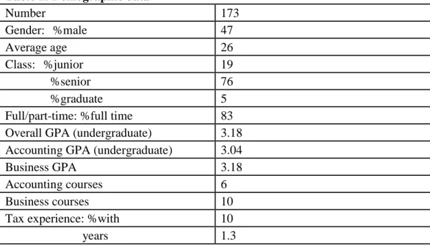
The subjects were 173 students enrolled in an undergraduate tax course. As can be seen from Table 1, the mean age of the students was 26. They were generally full-time students (86%) and only 10% had had any practical tax experience.
Table 1: Demographic data
Number 173
Gender: %male 47
Average age 26
Class: %junior 19
%senior 76
%graduate 5
Full/part-time: %full time 83 Overall GPA (undergraduate) 3.18 Accounting GPA (undergraduate) 3.04
Business GPA 3.18
Accounting courses 6
Business courses 10
Tax experience: %with 10
years 1.3
Design
The participants were given a booklet containing an introductory letter, the experimental instrument and a post-test questionnaire. The experimental task required the participant to decide whether an individual taxpayer could be regarded as a "dealer" or "investor" in real property. This specific task was chosen as it is often decided by taking into account the facts and circumstances of the taxpayer's situation.
The subject matter of the task has well-defined criteria from which it was possible to obtain information sets of different lengths. The criteria are such that they could be constructed into positive or negative cues. Although this is a typical tax research task, it is unlikely that it is one about which the students would have had strong priors. This subject matter has been used in other studies (e.g., Roark and Reneau, 1989; Pei et al., 1990, 1992).
The cues used in this study were based on the set of cues developed by Taylor (1980) from the relevant case law. The cues were ranked and scaled as to their importance in an "investor - dealer"
decision by a group of experienced tax Ph.D. students and tax faculty at a major state university.2 The cues were constructed from the results of this exercise. The positive and negative cues were made approximately equal in strength. The cues regarded to be the most important were in each cue level, as these are more likely to be influential in the decision making process. The less important cues were added for the longer cue levels. This was done as it is expected that the more important cues would be used first in any summary of facts. (This may give a slight bias against the prediction of recency). The cues were designed to be unambiguously positive or negative. The initial belief was anchored at 50 percent.
This was accomplished by indicating, before the cues were seen, that there was a 50:50 chance of either
2 The Ph.D. students had had experience as tax managers, just prior to entering the Ph. D. program.
Two were advising some private clients. The tax faculty were generally less experienced.
treatment. The instrument presented the client facts and the results of the staff member's "research."
The subjects were asked to make a series of sequential decisions as new client facts were received. In order to force the subjects to encode the information in a SbS process, each new client fact was presented on a new page. The decisions were requested on a 100 point scale placed at the bottom of each page.
The subjects were asked to mark on the scale what they believed to be the probability that the "client"
would be regarded as a "dealer" or an "investor" in real property.
The experiment was designed as a 2 x 3 ANOVA (Analysis of Variance). A between-subjects design was chosen because there was a major concern for the possibility of a carry-over effect in a cognitively complex sequential processing task. There was also a concern that, in a within-subject design, the subjects might have been able to guess the hypotheses (Pany and Reckers, 1987).
The subjects were randomly assigned to one of six (2x3) conditions. They were given as much time as they needed to discount time pressure as a variable.
Independent variables
There were two independent variables: order ("ORDER"), and the number of cues ("LOAD"). The ORDER factor had two levels: a) positive cues followed by negative ones (Level 1) and b) negative cues followed by positive ones (Level 2).3 The LOAD factor had three levels: a) four cues, b) eight cues, and c) twelve cues. These cue lengths were chosen to bracket seven (Miller, 1956), and because it was considered unlikely that a client's facts would have many more than twelve separate items of information for any single legal tax research task.
Dependent variable
The dependent variable was the change in belief from the manipulated anchor. That is, the belief after all items of information have been received less the initial anchor of 50%.
4. Data analysis
Hypothesis I
The analysis was conducted using a 2x3 ANOVA. The results of the analysis are shown in Table 2.
3 There is often some concern that the serial position of the cues could affect judgments. Therefore, the cues within each directional series were presented in two different orders so that any serial effects could be observed. It should be noted that the model assumes that there is no serial effect. A serial effect was tested for, but was not found. This confirmed Pei et al. (1992) who also did not find a serial effect.
Table 2
ANOVA table for two-way analysis
Source DF SS F value P value
Model 5 9831.94 3.11 0.0104
Error 167 105740.00
Source DF SS III F value P value
Order (O) 1 5009.57 7.91 0.0055
Load (L) 2 2396.56 1.89 0.1539
L * O 2 2655.61 2.10 0.1260
Because the results show that there is no interaction, it is permissible to look at the main effects.
There is a significant main effect for ORDER (p = 0.006). The overall means of the two levels of the factor indicate that there is a recency effect. Therefore, the evidence is again consistent with the predictions of hypothesis I.
Hypothesis II
Hypothesis II stated that the recency effect is expected to diminish as the number of cues in the series increases.
Two-way ANOVA results. The analysis was conducted using the same 2x3 ANOVA model used to test hypothesis I. If the results were consistent with the prediction of hypothesis II, one would expect to see a significant LOAD by ORDER interaction. The results are reported in Table 4. The results show that the LOAD by ORDER interactions are not significant in either case. Thus, the evidence is not consistent with the prediction of hypothesis II.
From a practical viewpoint, it was considered important to obtain further insight into the effect of increasing the LOAD levels. Therefore, multiple pairwise comparisons were analyzed.4 This analysis showed that the mean of the twelve cue LOAD factor in ORDER level 1 (+ -) was significantly different from the mean of the twelve cue LOAD level in ORDER level 2 (- +) and from the mean of the eight cue LOAD level in ORDER level 2 (- +). No other pairwise comparisons were significant. The multiple pairwise comparisons suggest that there may be a difference in the ORDER effects among the different LOAD factor levels but not in the pattern predicted by hypothesis II.
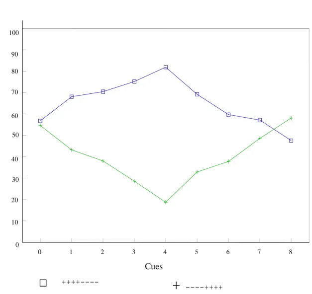
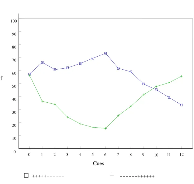
The table above and the figures below (figures 2-4) show that as the number of cues increase the
“fish-tail” effect (recency bias) becomes more pronounced. The four cue series results show no recency effect, whereas the twelve cues series shows a significant recency effect (the eight cue series shows a moderate recency effect). Looking at the figures, it can be seen that for the four cue series there is no
“fish-tail” effect – the beliefs after the fourth cue are almost the same for the two ORDERs (positive – negative; and negative – positive). Figure 3 has a slight “fish-tail”, the lines for the two ORDERs cross
4 Scheffé's method was used.
just before the final cue. Figure 4 shows a substantial “fish-tail” effect, the crossover of ORDER lines is before the tenth cue.
Figure 2 Four cue series
Cues Belief
0 1 2 3 4
100 90 80 70
60 50 40 30 20
10 0
++-
- + --++
Figure 3 Eight cue series
Cues Belief
0 1 2 3 4 5 6 7 8
100
90 80 70
60 50
40 30 20
10
0
+
----++++++++----
Figure 4 Twelve cue series
One-way ANOVA results. As a result of the analysis reported in the previous subsection, it was considered appropriate to partition the data by LOAD factor levels and to analyze the partitioned datasets in three separate one-way ANOVAs. The results are shown in Table 3.
Cues Belief
0 1 2 3 4 5 6 7 8 9 10 11 12
100
90 80 70 60 50 40
30 20 10
0
+++++---
+
---++++++Table 3
ANOVA tables for one-way analysis Four cue load
Source DF SS F value P value
Model 1 26.67 0.05 0.8262
Error 58 31800.73
Eight cue load
Source DF SS F value P value
Model 1 1564.57 2.42 0.1254
Error 54 34868.86
Twelve cue load
Source DF SS F value P value
Model 1 5927.17 8.34 0.0055
Error 55 39070.41
These results indicate that there is a highly insignificant difference in the cell means for the four cue LOAD level (p = 0.826), a mildly insignificant difference in the cell means for the eight cue LOAD level (p = 0.125) and a highly significant difference in the cell means for the twelve cue LOAD level (p = 0.006).
This suggests that there is a strong ORDER effect at the twelve cue LOAD level. Inspection of the cell means shows that they are consistent with a recency effect. Since, as stated above, the weaker cues were added for the longer series, the fact that a recency effect was found in the longer series indicates the strength of the recency bias.
Summary. Hypothesis II predicted a significant LOAD by ORDER interaction in the two-way ANOVA. None was found. Thus, the evidence is not consistent with the prediction of hypothesis II.
However, the multiple pairwise comparisons indicate that there were differential order effects among the LOAD levels. Based on analyses using one-way ANOVAs, the results indicate that the strength of the
recency effect increases as the number of cues in the series increases. The twelve cues LOAD series being significant, whereas the four cues LOAD series is insignificant. This is opposite to the prediction of hypothesis II.
5. Discussion and limitations
Discussion
From the analysis section above it can be seen that a strong recency order effect was found. This is consistent with the predictions of the Belief Adjustment model. However, the multiple pairwise comparisons in the two-way ANOVA and the one-way ANOVA results of the individual LOAD levels suggest that the strong recency order effects may be driven mainly by the longer cue LOAD level.
The strength of the recency order effect in the twelve cue LOAD factor level may indicate that Hogarth and Einhorn (1992) were justified in stating that a series of twelve cues could be regarded as a short series. If this is the case, then the Butt and Campbell (1989) study does not support the model.
Further, Hogarth and Einhorn's (1992) statement that Butt and Campbell's series of ten cues was more like a long series may not be justified.
Considering that most of the prior studies have found strong recency effects, the lack of a significant effect for the four cue LOAD factor level is surprising. However, the insignificant results found in this study for the four cue LOAD level are not inconsistent with the results previously found for inexperienced tax managers (Pei et al., 1992). Thus, it is possible that inexperienced tax decision makers, such as students, are cautious when they have a small number of cues available and so are able to show more consistent evaluations. As the number of cues increases, the bias that the model predicts may become influential. Further research is needed to establish the demarkation between a short and a long series.
The strong recency order effect found in the longer cue series should be of interest to the tax profession. As stated earlier, tax advisors, typically, are likely to use more than a small number of cues in their judgments. In these cases, the recency order effect may result in a systemic bias in their judgments.
It would be of benefit to tax advisors if they are made aware of this potential bias, so that they may be able to undertake measures designed to prevent the bias from occurring.
Appropriate measures could include the mixing of evidence of different directions before it is analyzed. This would be possible where the advisor uses an electronic database (or a hard copy tax service) to search for, say, relevant court cases. The database usually provides the researcher with a brief summary of the findings of the case. This enables the researcher to judge whether that particular case supports or contradicts his intended position.
Limitations
The experiments were carried out together in a laboratory setting. This is a different environment to the one in which students would normally carry out their research. The subjects were undergraduate students taking a tax course at a major western public university. Although there is no evidence that these students' cognitive processes would be different from those of other students, generalization to all tax students may be limited. Thus, there are some serious concerns about the external validity of this experiment.
The subjects were given the different instruments at the same time. They were told that the instruments were designed to take different amount of time to complete and that they should expect that some would be finished before others. However, it is possible that some subjects with the longer
instruments may have rushed their tasks and did not give considered responses.
Future research should be able to look at different techniques to mitigate the order biases found in this research to ascertain which techniques are efficient and under what conditions such techniques do counter the order bias potential in tax decisions. Further research could include using mixed positive and negative cue alternatively to ascertain whether this would mitigate the recency bias.
6. Summary
The Belief Adjustment model predicts recency effects for complex information encoded in a step-by-step process. Prior studies using the model in a tax context have examined balanced information sets of two or four cues and have generally used professionals. Generally, these studies found a recency effect. However, psychology literature indicates that the recency effect may not carry-over to long series of cues.
This study extended prior work by looking at students and different number of cues. It investigated the effect of series of four, eight, and twelve cues on tax research decisions. An experiment was carried out. The subjects were 173 undergraduate students enrolled in tax courses at a major U.S. state university.
It was found that there was a strong overall recency order effect. However, the recency order effect was driven by the longer cue series, rather than by the shorter cue series. This is contrary to the predictions of the Belief Adjustment model.
Students under taking tax research generally use a fairly large number of items of information in their judgments. Thus, the finding of a strong recency order effect in the longer series should be of interest to tax educators. Tax educators should be able to teach students to avoid the possibility of succumbing to order biases during tax research tasks. This training then should carry over to the time when the students become professionals.
References
Anderson, N.H. 1981. Foundations of Information Integration Theory. Academic Press. New York.
Asare, S.K., 1992. The auditor's going concern decision: Interaction of task variables and the sequential processing of evidence. Accounting Review 67, 379-393.
Asare, S.K. and Messier, W.F, 1991. A review of audit research using the Belief Adjustment model.
In: L. Ponemon and D.R. Gebhart (Eds), Auditing; Advances in Behavioral Research:
Springer-Verlag, New York .
Ashton, A.H., R.H. Ashton R.H., 1988. Sequential belief revision in auditing. The Accounting Review 63, 623-641.
Butler, S.A., 1986 Anchoring in the judgmental evaluation of audit samples. The Accounting Review 61, 101-111.
Butt, J. L., Campbell, T.L., 1989. The effects of information order and hypothesis testing strategies in auditor's judgments. Accounting, Organizations and Society 14, 471-479.
Christian, C.W., Reneau, J.H., 1989. Updating beliefs in legal tax research. An experimental test of the belief adjustment model. Unpublished manuscript, Arizona State University.
Gibbins, S.M., 1984. Propositions about the psychology of professional judgment in public accounting.
Journal of Accounting Research 22, 103-125.
Hogarth, R.M., 1987 Judgment and choice. John Wiley, Chichester, West Sussex.
Hogarth, R.M., Einhorn, H.J., 1990 Order effects in belief updating: The Belief Adjustment model.
Working Paper.Graduate School of Business, University of Chicago.
Hogarth, R.M., Einhorn, H.J., 1992 Order effects in belief updating: The Belief Adjustment model.
Cognitive Psychology 24, 1-55.
Johnson, L., 1993 An empirical investigation of the effects of advocacy on preparers’ evaluations of judicial evidence. Journal of the American Taxation Association 15,1-21.
Kahneman, D., Tversky, A., 1972 Subjective probability: A judgment of representativeness.
Cognitive Psychology 3,430-454.
Kahneman, D., Tversky, A., 1979. Prospect theory: An analysis of decision under risk.
Econometrica 47, 263-291.
Knechel, W.R., Messier, W.F., 1990. Sequential auditor decision making: Information search and
evidence evaluation. Contemporary Accounting Research 6, 386-406.
Markowitz, H., 1952. The utility of wealth. Journal of Political Economy 60, 151-158.
Messier, W.F., 1992. The sequencing of audit evidence: Its impact on the extent of audit testing and report formulation. Accounting and Business Research, 22, 143-150
Messier, W.F., Tubbs, R.M., 1994. Recency effects in belief revision, the impact of audit experience and the review process. Auditing: a Journal of Practice and Theory, 13, 57-72.
Miller, G.A., 1956. The magic number seven plus or minus two. Some limits on our capacity for processing information. Psychological Review 63, 81-97.
Murdock, B.B. 1962. The serial position effect in free recall. Journal of Experimental Psychology, 64, 482-488.
Pany, K. , Reckers, P.M.J., 1987. Within vs. Between – subjects experimental designs; a study of demand effects. Auditing: a Journal of Practice and Theory 7, 39-53.
Pei, B.K.W., Reckers, P.M.J., Wyndelts, R.W., 1992. Tax professionals' belief revision: The effect of information presentation sequence, client preference and domain experience. Decision Science. 23, 175-199.
Pei, B.K.W., Reckers, P.M.J., Wyndelts, R.W., 1990, The influence of alternative information on professional tax judgments. Journal of Economic Psychology 11, 119-146.
Pennington, N., & Hastie, R. 1986. Evidence evaluation in complex decision making. Journal of Personality and Social Psychology, 51, 242-258.
Robinson, L.B., & Hastie, R. 1985. Revision of beliefs when a hypothesis is eliminated from consideration. Journal of Experimental Psychology: Human Perception and Performance, 11, 443-456.
Roark, S.J., Reneau, H.J., 1989. An experimental test of factors affecting tax advisor's information acquisition and recommendations. Unpublished manuscript, Arizona State University.
Taylor, R.L., 1980. Dealers and investors in real estate. Journal of Real Estate Taxation, 7, 395-403.
Tubbs, R.M., Messier, W.F, Knechel, W.R., 1990. Recency effects in the auditor's belief revision process. The Accounting Review, 65, 452-460.
Tversky, A., Kahneman D.,1974. Judgment under uncertainty: Heuristics and biases. Science 185, 1124-1131.
Copyright Disclaimer
Copyright reserved by the author(s).
This article is an open-access article distributed under the terms and conditions of the
Creative Commons Attribution license (http://creativecommons.org/licenses/by/3.0/).