Vol. 18, No. 4, 2003, 402 - 417
THE DILUTION EFFECT OF ACCOUNTING INFORMATION
1Jogiyanto Hartono Universitas Gadjah Mada
ABSTRAK
Riset ini meneliti efek gabungan antara kejutan-kejutan dividen dan laba. Dengan menggunakan belief-adjustment theory yang dikenalkan oleh Hogarth and Einhorn’s (1992), riset ini menguji perilaku dari reaksi investor terhadap waktu (timing) dari pengumuman-pengumuman dividen dan laba. Teori ini memprediksi bahwa untuk kejutan-kejutan konsisten yang terjadi pada waktu bersamaan, mereka mempunyai pengaruh yang lebih kecil di return saham dibandingkan dengan kejutan-kejutan konsisten yang terjadi secara berurutan (hipotesis ini disebut dengan hipotesis efek dilusi atau the dilution effect hypothesis).
Hipotesis-hipotesis efek dilusi ini didukung di satu dari empat skenario yaitu terjadi pada waktu kejutan-kejutan laba positip. Hipotesis-hipotesis ini tidak didukung untuk kejutan-kejutan dividen negatip, kejutan-kejutan dividen positip dan kejutan-kejutan laba negatip.
Key words: the dilution effect, belief adjustment theory, belief revision, Hogarth and Einhorn, behavioral finance, behavioral accounting, behavioral market research, contemporaneous announcements, simultaneous announcements, joint announcements, noncontemporaneous announcements, sequential announcements, mixed evidence, consistent evidence.
1 This study is a part of my dissertation. I am very grateful to Dr. Roland Lipka, Dr. Heibatollah Sami, Dr. David Ryan and Dr. Michael Goetz for their insightful comments and guidance. I also acknowledge the helpful suggestions from Dr. Sharad Asthana and Dr. Steven Balsam. Financial support was provided by a Summer Research Fellowship Award at Temple University.
INTRODUCTION
Hartono (2004a) found evidence of recency effect of a sequential orderly accounting information. He found that when dividend and earnings surprises are considered together, only positive dividend surprises that follow negative earnings surprises create a combined recency effect. This means that the order of positive dividend surprises that follow negative earnings surprises has a greater positive effect on stock returns than when the order is reversed.
Hartono (2004b) also found evidence of ‟no-order effect‟ of a sequential orderly accounting information. He found that for consistent positive evidence (good news followed by another good news), the order of surprises whether the positive dividend surprise follows or precedes a positive earnings surprise does not matter.
question of how order of the information can change investors‟ belief about stock prices. The latter more focuses on the timing of the information to answer the question of when timing, contemporaneously or sequentially, of the information can change investors‟ belief about stock prices.
While order is defined as the sequence of the surprises whether dividend surprises precede or follow earnings surprises and whether bad news precedes or follows good news,2 timing is defined as the interval between two announcement dates. Eddy and Seifert (1992) defined two announcements as contemporaneous announcements (simulta-neous announcements or joint announcements) if they occur within two trading days, whereas noncontemporaneous announcements (sequential announcements) are those that are separated by more than two trading days. In this study, simultaneous announcements are defined when two surprises occur on the same day.
Therefore, this study addresses the issue of when investors revise their belief to stock prices, whether they react on contemporaneous announcements or on sequential announ-cement. Using Hogarth and Einhorn's (1992) belief-adjustment theory, this study predicts that for consistent evidence when dividend and earnings surprises occur at the same time, they have less impact on stock returns than when they occur sequentially (dilution effect hypothesis).
Hogarth and Einhorn's (1992) belief-adjustment theory is used in this study to test the behavior of investors‟ reaction to the timing of dividend and earnings surprises. The objective of this dissertation is to test the dilution effect hypothesis using accounting information to determine whether individual behavior as predicted by the theory is
2 The terms surprise, evidence, news and unexpected change are used interchangeably in this study.
consistent with the aggregate behavior of investors.
THEORY AND HYPOTHESES DEVELOPMENT
The Belief-Adjustment Theory
Beliefs are the critical component in the decision making process (Beaver 1989). The level of beliefs determines decision making behavior. The role of information is to alter beliefs. Therefore, decision making behavior is altered when newly arrived information changes beliefs. Beaver (1989), using this argument, also stated that the role of accounting information is to alter the beliefs of investors.3 Investor beliefs are unobservable. Stock prices can be viewed as arising from an equilibrium process of investors' beliefs (Bamber 1987; Lev 1988; Beaver 1989; Kim and Verrecchia 1991; and Bamber and Cheon 1995).4
Dividend and earnings surprises are chosen because not only are they individually important accounting information but they also possess characteristics that can alter beliefs. The timing of dividend and earnings surprises varies. Some companies routinely announce dividend and earnings surprises simulta-neously. Other companies make the announ-cements separately. The question thus arises as to whether the presentations of timing of dividend and earnings surprises can alter investors‟ beliefs differently.
Application of the theory in this study may expand our understanding of when two different pieces of accounting information
3 The use of the term investors as shareholders is consistent with the primary user orientation of FASB (1978). Other groups of users are bondholders, corporate raiders, and suppliers, among others.
4 There is a conceptual difference between stock price and trading volume. While price changes reflect changes in
the aggregate market‟s average beliefs; in contrast,
trading volume is the sum of all individual investors‟
jointly considered by investors may affect their beliefs. In accounting settings, the theory has been applied in auditing (for example, Ashton and Ashton 1988, 1990; and McMillan and White 1993), in management accounting (Dillard et al. 1991) and in taxation (Pei et al. 1990), but not in financial market studies.
Because of differences in type, order and timing of evidence, belief-adjustment theory predicts different effects in belief adjustment. The type of evidence is determined by whether all of the evidence is in the same direction (consistent evidence) or not (mixed evidence). Recall that the definition of evidence is an unexpected change (surprise) in value of dividends or earnings. Consistent evidence is a series of surprises that have the same direction, either all positive (increasing value) or all negative (decreasing value). Mixed evidence is a series of negative and positive surprises. Order classifies the sequence of evidence. It distinguishes between dividend surprises followed by and preceding earnings surprises (DE versus ED, where D and E stand for dividend and earnings surprises, respectively), and between negative surprises and positive surprises. Timing of evidence refers to the mode of evidence whether surprises are presented sequentially or simultaneously.
The belief-adjustment model can be formu-lated as follows (Hogarth and Einhorn 1992).
Bk = Bk-1 + wkEk(d), (1) Where:
Bk = current belief about stock price after evaluating k pieces of dividend and, or earnings evidence,
Bk-1 = anchor or prior belief about stock price,
wk = the adjustment weight for the kth piece of dividend or earnings evidence, Ek(d) = magnitude of the kth piece of dividend
or earnings evidence,
d = the direction of the evidence, whether it is negative or positive evidence.
Evidence or a surprise is defined as a change in value of dividends or earnings from prior to current quarters. The value of the adjustment weight, wk, depends on the direction of the evidence. Hogarth and Einhorn (1992) argued that for negative evidence, Ek(-), the adjustment weight (wk) is specified as proportional to the anchor (Bk-1):
wk = Bk-1 for 0 < 1. (2a) This argument implies an effect called the contrast effect: larger anchors (Bk-1) are "hurt" more than smaller ones by the same negative evidence. Hogarth and Einhorn (1992) gave a rationale for this treatment as follows. The same negative evidence causes a larger reduction in high anchors than it does in low anchors. They argued that it is the behavior of the people who have a tendency to perceive that low anchors are already low and will not reduce them as much as if the anchors are high.
With the same argument, it is assumed that for positive evidence, wk is inversely proportional to the anchor or in other words, the same positive evidence increases more for small anchors than it does for large anchors (Hogarth and Einhorn 1992):
wk = (1-Bk-1) for 0 ß < 1. (2b) The adjustment weight is also affected by one's sensitivity toward negative or positive evidence, and , respectively. Values of =1 and =1 indicate high sensitivity to negative and positive evidence, respectively. Similarly, =0 and =0 indicate no sensitivity to negative and positive evidence, respectively.5
Substituting equation (2a) and (2b) into equation (1) yields:
Bk = Bk-1 + Bk-1Ek(-), and (3a) Bk = Bk-1 + (1 - Bk-1)Ek(+). (3b)
Equation (3a) refers to a belief-adjustment model for negative evidence and equation (3b) refers to a belief-adjustment model for positive evidence.
Two response modes are recognized by the belief-adjustment theory: the Step-by-Step (SbS) and the End-of-Sequence (EoS). In the SbS, evidence is presented and evaluated sequentially, while in the EoS, evidence is presented and evaluated simultaneously or at once. Under the condition that attitudes toward evidence are sensitive, sequential presentation of consistent evidence will yield greater belief revision than will simultaneous presentation of consistent evidence. This effect is called the dilution effect in simultaneous processing (Ashton and Ashton 1988).
DEVELOPMENT OF HYPOTHESES
A dilution effect is predicted for simultaneous, consistent evidence. It suggests that the effect of simultaneous evidence on the belief adjustment is smaller than that of sequential evidence (Ashton and Ashton 1988). Studies in experimental psychology using accounting settings (Ashton and Ashton 1988; McMillan and White 1993; Dillard et al. 1991; and Pei et al. 1990) supported the predictions of the theory. This study tests the theory whether such behavior holds for share price data at the market level.
The issue of whether dividend and earnings surprises are interactive when they are announced jointly was not formally addressed until the Kane et al. (1984) study. This study used 352 observations of quarterly earnings and dividend surprises that occurred within 10 days of each other between the fourth quarter of 1979 and the second quarter of 1981. A naive dividend expectation model and the Box-Jenkin's earnings expectation model were used. Cumulative abnormal returns were calculated for days -10 to +10 using a market model. This study found that both earnings and dividends convey information. Including dummies that represent the signs of dividend and earnings
surprises made the earnings and dividend coefficients insignificant, but left the dummies significant. They concluded that a corroborative effect exists between earnings and dividend surprises in the sense that markets interpret surprises in relationship to each other.6
Chang and Chen (1991) reexamined the Kane et al. (1984) study. They used a sample of 2,688 earnings and dividend announcements from 1981 to 1984. Initially, they used the same methods employed in Kane et al. They found support for the corroborative effect. But they suspected that the long event window (30 days) used by Kane et al. might account for the effect. So, they conducted tests to vary the interval between announcements and the length of CAR windows. They did not find any systematic patterns of earnings effect, dividend effect and corroborative effect across different intervals. The interaction dummies were only significant when the CAR windows were more than 10 days. They concluded that the corroborative effect did not exist and that the Kane et al. finding was due to corporate noise (other events) within the long window interval.
Leftwich and Zmijewski (1994) also conducted a joint study of dividend and earnings surprises. Their focus was on contemporaneous announcements. The contem-poraneous announcements were identified
6 Freeman and Tse (1989) extended the analysis of corroborative effect to earnings postannouncement events. They argued that additional postannouncement information causes investors to adjust their belief regarding the permanent nature of earnings. They
defined two type of corroboration news: “confirmed earnings” (an increase in both previous quarter and
current quarter random walk forecast errors) and
“contradicted earnings” (a different sign of random walk
when the CRSP dividend declaration dates and Compustat earnings announcement dates were within the same trading day of each other. Their final sample consisted of 972 observations from 1977 to 1987. Three-day excess returns were regressed on earnings forecast error and the dividend forecast error. The coefficients from the earnings and dividend forecast errors were 0.490 (t statistic of 4.03) and 2.412 (t statistic of 2.99), respectively. They concluded, without presenting statistical evidence, that quarterly dividend surprises conveyed information beyond that contained in contemporaneous quarterly earnings surprises. Considering the signs of the surprises, their univariate tests showed that when there is no dividend surprises, the negative and positive earnings surprises earned excess returns of 0.68 percent and 0.46 percent, respectively. On the contrary, if there is no earnings surprise, none of the dividend surprises produced excess returns that were statistically greater than zero. Further, Leftwich and Zmijewski regressed the excess returns on six dividend and six earnings interaction variables. The interactions variables represent interaction between the magnitude of the dividends or earnings and their signs (positive, zero or negative forecast errors). From the six dividend coefficients, only one coefficient for positive earnings and negative dividend surprises was reliably greater than zero. All six coefficients for the earnings interaction variables were statistically greater than zero. From these results, again without comparing them statistically, they concluded that earnings provide information beyond that provided by dividends, especially when dividends and earnings provide consistent surprises or when dividends provide no surprise. Since this study focused only on the contemporaneous announcements, the order of surprises, whether dividend surprises follow or precede earnings surprises or whether good news follows or precedes bad news was not investigated.
Eddy and Seifert (1992) also investigated the joint effects of dividend and earnings surprises. They defined announcements as joint announcements if they occurred within two trading days of each other. They used a sample of 1,111 firms from 1983 to 1985. The naive dividend expectation model and the Value Line analyst's earnings forecast model were used. They found that dividend and earnings surprise effects were not substitutes for each other. This means that the effects of joint surprises in
contemporaneous (simultaneous)
announcements and single surprise in noncontemporaneous (sequential) announ-cements are different. From their univariate test, they found that stock price reactions were significantly greater for contemporaneous consistent positive surprises than those for single noncontemporaneous surprises. Eddy and Seifert (1992) compared the means price reaction of the two types of announcements. Based on the univariate test, they found that the reaction to joint dividend and earnings surprises was significantly higher than the reaction of a single dividend or earnings surprises announced separately by more than two days. This result was not surprising since they compared the effect of two pieces of evidence to that of only one piece of evidence. Other things equal, of course, the former will yield a greater effect than the latter. Had they compared the mean price reaction of joint dividend and earnings surprises to that of two single surprises added together, the result could be different. The belief-adjustment theory predicts that the former will yield a smaller effect (dilution effect) than the latter.
The dilution effect can be demonstrated as follows. For consistent evidence, consider again the basic model in equations (3a) and (3b). For first evidence, the equations can be written as:
B1- = B0 + B0E1(-)
After consistent second evidence, equations (3a) and (3b) can be written as:
B-,-2 = B1- + B1- E2(-)
= B1- 1 + E2(-)], and (5a) B+,+2 = B+1 + 1 - B+1 )E2(+). (5b) For the consistent negative evidence, substituting B1- from equation (4a) into equation (5a) will yield:
B-,-2 = B01 + E1(-)] [1 + E2(-)] (6a) When two pieces of negative evidence are presented sequentially, from equation (6a), the final belief becomes:
B-,-2 = B0[1 + E1(-)] [1 + E2(-)] = B0[1 + E1(-) + E2(-) + E1(-)E2(-)]
= B0 + B0[E1(-) + E2(-) + E1(-)E2(-)].
For simultaneous presentation of consistent evidence, Ashton and Ashton (1988) argued that information is evaluated as a whole based on the accretion model as follows:
E*2(-) = E1(-) + E2(-) + E1(-)E2(-). (7) When two pieces of negative evidence are presented simultaneously, from equation (3a), the final belief is:
B*-,-2 = B0 + B0 E*2(-)
= B0 + B0[E1(-) + E2(-) + E1(-)E2(-)].
The difference between belief resulting from sequential consistent evidence and that from simultaneous consistent evidence is the size of the dilution effect, which can be stated as follows:
B-,-2 - B*-,-2 = B0 + B0E1(-) + B0E2(-) +
B0E1(-)E2(-) –
B0 - B0E1(-) - B0E2(-) – B0E1(-)E2(-)
= B0E1(-)E2(-) – B0E1(-)E2(-)
= B0E1(-)E2(-)( - 1). (8) Since 0 < 1, i.e., one's attitude toward negative evidence is disconfirmation prone (sensitive toward negative evidence), ( - 1) is negative. Therefore B-,-2 - B*-,-2 is negative. This result shows that for negative consistent evidence, the negative impact of sequential processing on the final belief is greater than that of simultaneous processing.7 This dilution effect indicates that simultaneous processing weakens the impact of the negative evidence.
The dilution effect in simultaneous pro-cessing also occurs for consistent positive evidence. When two pieces of positive evidence are presented sequentially, from equation (5b), the final belief is:
B+,+2 = B0 + 1 - B0)[E1(+) + E2(+) – E1(+)E2(+)]
= B0 + 1 - B0)E1(+) + 1 - B0)E2(+) – 1 - B0)E1(+)E2(+).
7 For example, assume that the initial stock price (B 0) is $10; that strengths of the evidence are 0.2 and 0.3 for first negative evidence, E1(-), and second negative evidence, E2(-), respectively; and that investor sensi-tivity toward negative evidence, , is 0.5. If evidence is
presented sequentially, the new stock price, B-,-2 , will be $10 + $10[(0.5)( 0.2) + (0.5)( 0.3) + (0.5)(
0.2)(0.5)( 0.3)] = $7.65. The change of initial and new prices is $7.65 - $10 = $2.35. If negative evidence
is presented simultaneously, the new stock price, B*-,-2 , will be $10 + (0.5)($10)[( 0.2) + (0.3) + (0.2)(
When two pieces of positive evidence are presented simultaneously, from equation (3b), the final belief becomes:
B*+,+2 = B0 + 1 - B0)E*2(+)
= B0 + 1 - B0)[E1(+) + E2(+) – E1(+)E2(+)]
= B0 + 1 - B0)E1(+) + 1 - B0)E2(+) – 1 - B0)E1(+)E2(+). The difference between the two beliefs is:
B+,+2 - B*+,+2 = - 1 - B0)E1(+)E2(+) + 1 - B0)E1(+)E2(+) = (1 - B0)E1(+)E2(+)(1 - ).
…..(9) Since 0 < 1, i.e., one's attitude toward positive evidence is confirmation prone (sensitive toward positive evidence), (1 - ) is positive. Therefore B+,+2 - B*+,+2 is positive. This suggests that for positive consistent evidence, the positive impact of sequential processing on the final belief is greater than that of simultaneous processing. The dilution effect in simultaneous processing of consistent positive evidence weakens the impact of the positive evidence.
The results of the dilution effect lead to the following hypotheses:
H1 The dividend response coefficient of a negative dividend surprise is smaller for simultaneous consistent negative evidence than the dividend response coefficient of a negative dividend surprise for sequen-tial consistent negative evidence.
H2 The earnings response coefficient of a negative earnings surprise is smaller for simultaneous consistent negative evidence than the earnings response coefficient of a negative earnings surprise for sequential consistent negative evidence.
H3 The dividend response coefficient of a positive dividend surprise is smaller for simultaneous consistent positive evidence than the dividend response coefficient of a positive dividend surprise for sequential consistent positive evidence.
H4 The earnings response coefficient of a positive earnings surprise is smaller for simultaneous consistent positive evidence than the earnings response coefficient of a positive earnings surprise for sequential consistent positive evidence.
METHODOLOGY
Sample Selection
payouts reduce the possibility that the changes were expected.
Announcement dates for the corresponding earnings per share are collected from Compustat tapes. Dividend announcement dates are collected from CRSP tapes. When dividends and earnings are announced on the same day, they are categorized as simultaneous
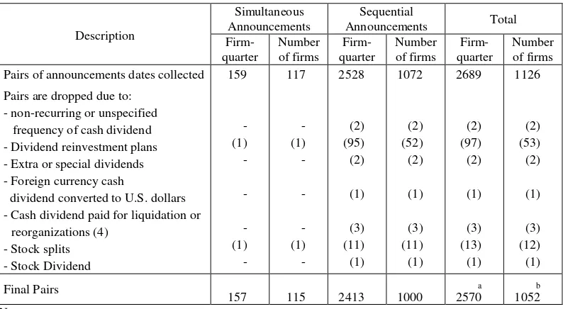
(joint or contemporaneous) announcements. When the interval is three or more days, they are considered as sequential (noncontem-poraneous) announcements. A total of 2,413 pairs of surprises are collected for sequential announcements and 157 pairs for simultaneous announcements. Table 1 shows the sample selection.
Table 1. Sample Selection Process
Description Pairs of announcements dates collected
Pairs are dropped due to: - non-recurring or unspecified frequency of cash dividend - Dividend reinvestment plans - Extra or special dividends - Foreign currency cash
dividend converted to U.S. dollars - Cash dividend paid for liquidation or
quarter at least one week late compared to their announcement date in year t-1. Investors‟ beliefs may be affected if they perceived that the late announcement was due to an auditing problem. Sensitivity analysis was conducted to test for any significant differences between late announcers and timely announcers. The results remain the same.
b The total number of firms should be 1115 (115 + 1000). The difference is due to the fact that the same 63
firms were included in both the simultaneous and sequential announcement groups.
Empirical Models
The following equations (10) and (11) are used to test the dilution effect hypotheses that simultaneous surprises have less impact on stock price changes than sequential surprises.
Where:
1. The dependent variables are MRRTSEQ and MRRTSIM. For the sequential group, MRRTSEQ is the average of the mean raw return for dividend and earning surprises. It is calculated as (MRRD + MRRE)/2. For the simultaneous group, MRRTSIM represents the mean of three-day raw returns (days -1, 0 and +1, for day 0 is the same dividend and earnings announcement day). MRRi for each firm is calculated as the mean of announcement date, respectively, for each firm.
2. MIMRT is the mean index of market returns and is explained below. This model is similar to the return models used by Ahmed (1994) and Kallapur (1994). MIMRT is the mean of the CRSP value-weighted index of market returns at the announcement date, one day before and one day after. The purpose of using MIMRT is to control for market factors that affect stock returns, such as interest rates or market risk premia (Kallapur 1994). Further, Kallapur used the market returns index to transform the raw announcements create noise in the measurement. To avoid this noise, days between two announcements are not used in the return calculation; rather, returns are calculated separately for each surprise.
returns in the dependent variable into market- and risk-adjusted returns.
3. Naive dividend and earnings expectation models are used to determine DPS and EPS.9 DPS (EPS) is calculated as the quarterly change in dividends (earnings) deflated by the last quarter stock price since it can reduce cross-section dependency bias (Christie 1987).
4. The dilution effect occurs in consistent evi-dence. Therefore, only interaction dummies for consistent evidence are included in the models. The dummy variable XSEQ(-,-) is the combination of dummies DE(-,-) and ED(-,-), while XSEQ(+,+) is the combination of dummies DE(+,+) and ED(+,+) for sequential announcements. For simultane-ous surprises, the dummy variable XSIM(-,-) is the combination of dummies DE(-,-) and ED(-,-), while XSIM(+,+) is the combination of dummies DE(+,+) and ED(+,+). The dilution effects occur when coefficients 2, 3, 4 and 5 are smaller than coefficients 2, 3, 4 and 5.
RESULTS
Descriptive Statistics of the Sample
The following table provides descriptive statistics for variables used in this study.
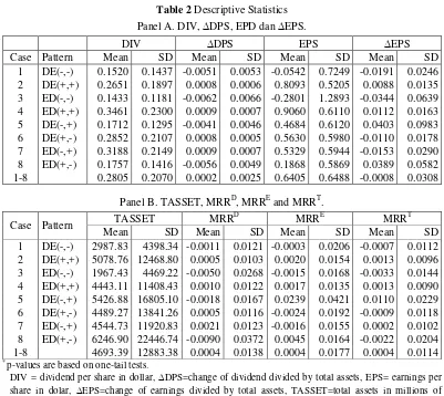
Table 2 Descriptive Statistics Panel A. DIV, DPS, EPD dan EPS.
DIV DPS EPS EPS
Case Pattern Mean SD Mean SD Mean SD Mean SD
1 DE(-,-) 0.1520 0.1437 -0.0051 0.0053 -0.0542 0.7249 -0.0191 0.0246 2 DE(+,+) 0.2651 0.1897 0.0008 0.0006 0.8093 0.5205 0.0088 0.0135 3 ED(-,-) 0.1433 0.1181 -0.0062 0.0066 -0.2801 1.2893 -0.0344 0.0639 4 ED(+,+) 0.3461 0.2300 0.0009 0.0007 0.9060 0.6110 0.0112 0.0163 5 DE(-,+) 0.1712 0.1295 -0.0041 0.0046 0.4684 0.6120 0.0403 0.0983 6 DE(+,-) 0.2852 0.2107 0.0008 0.0005 0.5630 0.5980 -0.0110 0.0178 7 ED(-,+) 0.3188 0.2149 0.0009 0.0007 0.5329 0.5944 -0.0153 0.0290 8 ED(+,-) 0.1757 0.1416 -0.0056 0.0049 0.1868 0.5869 0.0389 0.0582 1-8 0.2805 0.2070 0.0002 0.0025 0.6405 0.6488 -0.0008 0.0308
Panel B. TASSET, MRRD, MRRE and MRRT.
Case Pattern TASSET MRR
D
MRRE MRRT
Mean SD Mean SD Mean SD Mean SD
1 DE(-,-) 2987.83 4398.34 -0.0011 0.0121 -0.0003 0.0206 -0.0007 0.0112 2 DE(+,+) 5078.76 12468.80 0.0005 0.0103 0.0020 0.0154 0.0013 0.0096 3 ED(-,-) 1967.43 4469.22 -0.0050 0.0268 -0.0015 0.0168 -0.0033 0.0144 4 ED(+,+) 4443.11 11408.43 0.0010 0.0122 0.0017 0.0135 0.0013 0.0090 5 DE(-,+) 5426.88 16805.10 -0.0018 0.0167 0.0239 0.0421 0.0110 0.0229 6 DE(+,-) 4489.27 13841.26 0.0005 0.0116 -0.0024 0.0192 -0.0009 0.0118 7 ED(-,+) 4544.73 11920.83 0.0021 0.0123 -0.0016 0.0155 0.0002 0.0102 8 ED(+,-) 6246.90 22446.74 -0.0090 0.0372 0.0045 0.0164 -0.0022 0.0204 1-8 4693.39 12883.38 0.0004 0.0138 0.0004 0.0177 0.0004 0.0114 * p-values are based on one-tail tests.
DIV = dividend per share in dollar, DPS=change of dividend divided by total assets, EPS= earnings per share in dolar, EPS=change of earnings divided by total assets, TASSET=total assets in millions of dollars, MRRD=three-day mean raw return at dividend announcement date, MRRE=three-day mean raw return at earnings announcement date, MRRT=three-day mean raw return at dividend and earnings announcement dates.
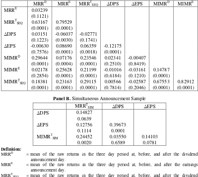
Diagnostics
The hypotheses are tested using ordinary least squares regressions. Diagnostics are conducted to ensure that the multicollinearity and heteroskedasticity problems do not bias the results. Multicollinearity occurs when two or more explanatory variables in the regression model are highly correlated. For the sequential sample, correlations between MIMRTSEQ and DPS, MIMRT
SEQ and EPS, and DPS and EPS are 0.00566, -0.02587 and -0.12175, respectively (see Panel A of Table 3). For the
that multicollinearity is not a serious problem in this study.
Table 3. Correlation Matrixes Panel A. Sequential Announcement Sample
MRRD MRRE MRRTSEQ DPS EPS MIMRD MIMRE MRRE 0.03239
(0.1121)
MRRTSEQ 0.63167 0.79529
(0.0001) (0.0001)
DPS 0.03151 -0.06037 -0.02771
(0.1223) (0.0030) (0.1741)
EPS -0.00630 0.08690 0.06359 -0.12175 (0.7576) (0.0001) (0.0018) (0.0001)
MIMRD 0.29644 0.07176 0.23546 0.02341 -0.00407 (0.0001) (0.0004) (0.0001) (0.2510) (0.8419)
MIMRE 0.02178 0.25628 0.21199 -0.01016 -0.03161 0.14787 (0.2854) (0.0001) (0.0001) (0.6184) (0.1210) (0.0001)
MIMRTSEQ 0.18381 0.23163 0.29115 0.00566 -0.02587 0.67553 0.82912 (0.0001) (0.0001) (0.0001) (0.7814) (0.2046) (0.0001) (0.0001)
Panel B. Simultaneous Announcement Sample
MRRTSIM DPS EPS
DPS 0.14827
0.0639
EPS 0.12756 0.39673
0.1114 0.0001
MIMRTSIM 0.24452 0.03550 0.14103
0.0020 0.6589 0.0781
Definition:
MRRD = mean of the raw returns in the three day period at, before, and after the dividend announcement day.
MRRE = mean of the raw returns in the three day period at, before, and after the earnings announcement day.
MRRTSEQ = mean of the raw returns in the three day period at, before, and after the dividend announcement day, and in the three day period at, before, and after the earnings announcement day.
MRRTSIM = mean of the raw returns in the three day period at, before, and after the simultaneous dividend and earnings announcement day.
MIMRD = mean of the CRSP value-weighted market returns in the three day period at, before, and after the dividend announcement day.
MIMRE = mean of the CRSP value-weighted market returns in the three day period at, before, and after the earnings announcement day.
MIMRTSEQ = mean of the CRSP value-weighted market returns in the three day period at, before, and after the dividend announcement day, and in the three day period at, before, and after the earnings announcement day.
MIMRTSIM = mean of the CRSP value-weighted market returns in the three day period at, before, and after the simultaneous dividend and earnings announcement day.
EPS = quarterly change of earnings deflated by prior quarter stock price (earnings surprises).
The use of deflators is one of the methods to correct the heteroskedasticity problem. Prior quarter stock prices is used as the deflator (Christie 1987). The remaining heteroskedasti-city is overcome using White‟s (1980) correction for heteroskedasticity.
Hypotheses Testing
Table 4 provides regression models to test the dilution effect hypotheses. The dilution effect only occurs for consistent evidence. Therefore, the regression models only consist of interaction dummies for consistent evidence as seen in equations (10) and (11). Models 1 and 2 in Table 4 are compared to test the dilution effect hypotheses for shorter intervals of sequential announcements. Model 1 is run using a sample where the interval between dividend and earnings announcements is 10 days or less, while model 2 is for intervals more than 10 days. A new variable called INTERVAL is added in model 3. INTERVAL contains values of intervals between dividend and earnings announcement dates, ranging from 3 to 90 days. The variable, INTERVAL, is an alternative test of the dilution effect. If the dilution effect exists for shorter intervals, the INTERVAL coefficient will be significantly positive which indicates that longer intervals have a greater effect on stock returns than shorter intervals. Model 3 is run using the full sample of sequential announcements. Model 4 is similar to model 3 but without INTERVAL variable. Model 5 is similar to model 4 but is run using the full sample of simultaneous announcements. Model 4 is compared to model 5 to test the dilution effect hypothesis of simultaneous announcement.
The dilution effect is tested by comparing two samples: the simultaneous announcement sample and the sequential announcement sample. Two groups of regressions are run: one for the simultaneous announcement sample (SIM) and another for the sequential announcement sample (SEQ). The hypothesis is tested using equations (10) and (11) Dummy variables used are X(-,-) instead of ED(-,-) and DE(-,-), and X(+,+) instead of ED(+,+) and DE(+,+). X(-,-) is the combination of ED(-,-) and DE(-,-). X(+,+) is the combination of ED(+,+) and DE(+,+).
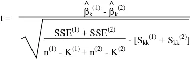
Hypothesis H1 posits that the effect of negative dividend surprises (DPS) on MRRT for consistent negative evidence is smaller for simultaneous announcements than that for sequential announcements. This hypothesis is, therefore, supported if coefficients 2 in equation (10) and 2 in equation (11) are not significantly negative and 2 is significantly smaller than 2. Model 5 in Table 4 shows that 2 is 0.189504 (insignificant), and model 4 shows that 2 is 0.032628 (insignificant). The t-test used to compare the coefficients between the (SIM) and (SEQ) samples appears in Hartono(1996) as follows:
t =
^ k
(1) - ^ k
(2)
SSE(1)+ SSE(2) n(1)- K(1) + n(2) - K(2)
[Skk(1) + Skk(2)]
The t-statistic that 2 < 2 is 0.226 which is insignificant for a one-tailed test. Therefore, H5a is not supported.
Table 4. Regression Results for Sequential and Simultaneous Announcements
Sequential
Simul-taneous t-test a)
1 2 t-test
a)
1 vs. 2 3 4 5 5 vs 4
NTERCEPT -0.000584 (-1.112)
-0.000937 (-2.178)**
-0.000606 (-1.402)
-0.000830 (-2.443)***
(-1.132) (-1.685)* (-1.533) (-1.952)** (-0.763)
Condition # 3.84587 3.63819 4.96073 3.69623 3.76077
F-Model 102.883 124.977 177.321 212.703 381.594***
1 = interval between dividend and earnings announcements is 10 days or less. 2 = interval between dividend and earnings announcements is more than 10 days. 3 = full sample for sequential announcements with INTERVAL variable. 4 = full sample for sequential announcements without INTERVAL variable. 5 = full sample for simultaneous announcements.
Notes:
- t-values in the parentheses. The first t-values are the unadjusted t-statistics. The second t-values are the
White‟s adjusted t-statistics.
- All condition numbers are less than 20 indicating multicollinearity is not a problem.
- Outliers are deleted by winsorizing based on two standard-deviations for dividend and earnings surprises and $5 of EPS.
- The descriptive statistics suggest that firm‟s size, which is defined as firm‟s total assets (TASSET), is different across cases. Including size variable (TASSET, TASSET per share or log of TASSET) does not change the results.
a) The t-test is based on the formula given in equation (A-5), see Appendix A.
** = significant at the 5% level. *** = significant at the 1% level.
Hypothesis H2 is similar to H1, but it is applied to negative earnings surprises (EPS). Hypothesis H2 is supported if coefficients 3 and 3 are not significantly negative and 3 is significantly smaller than 3. Coefficients 3 and 3 are 0.074847 (insignificant) and -0.002974 (insignificant), respectively. The t-statistic test of 3 < 3 is 1.022 which is insignificant for a one-tailed test. H2 is not supported.
Hypothesis H3 posits that the effect of positive dividend surprises (DPS) on MRRT for consistent positive evidence is smaller for simultaneous announcements than that for sequential announcements. Hypothesis H5c is supported if coefficients 4 and 4 are not significantly negative and 4 is significantly smaller than 4. Coefficients 4 and 4 are 0.194534 (insignificant) and 0.550784 (significant at the 10% level for a one-tailed test), respectively. The t-statistic test of 4 < 4 is -0.691 which is insignificant for a one-tailed test. Therefore, H3 is not supported.
Hypothesis H4 is similar to H3, but it is applied to positive earnings surprises (EPS). Hypothesis H4 is supported if coefficients 5 and 5 are not significantly negative and 5 is significantly smaller than 5. Coefficients 5 and 5 are -0.041393 (insignificant) and 0.031999 (significant at the 1% level for a one-tailed test), respectively. The t-statistic to test 5 < 5 is -1.947 which is significant at the 5% level for a one-tailed test. Both coefficients are not significantly negative. Therefore, H4 is supported.
Since simultaneous and sequential announ-cements differ only in the intervals, the dilution effects might also occur for shorter intervals of sequential announcements. To further test whether the interval itself contributes to the dilution effect, a new variable, INTERVAL, was added in the sequential announcement regression. This variable represents the actual number of days in the interval between the dividend and earnings announcement dates. If interval matters, its effect is expected to be positive, indicating that larger intervals have more effect on stock returns than shorter intervals. The result shows that INTERVAL is negative (-0.00001) and insignificant.
To further test the dilution effect for short intervals of sequential announcements, two sample groups were formed: the short interval group for stocks with intervals between dividend and earnings surprises less than or equal to 10 days, and the long interval group, for stocks with intervals more than 10 days. The cut-off point of 10 days is chosen because prior studies found that dividend and earnings announcements that were separated by more than 10 days had interaction effects. Models 1 and 2 in Table 4 show the regression results for shorter and longer interval groups, respectively. None of the t-statistics in comparing dividend and earnings response coefficients between shorter and longer intervals are significant, indicating that the dilution effect for short intervals of sequential announcements due to the magnitude of surprises does not exist.
SUMMARY AND DISCUSSION
The following Table 5 shows the summary of the hypotheses, their tests and their results. Table 5. Summary of Hypothesis Testing
Hypo- thesis
Direction of the evidence
Magnitude of the evidence
Order of the evidence
Test of
H5a Negative DPS (-,-) 2< 2 Not Supported
H5b Negative EPS (-,-) 3< 3 Not Supported
H5c Positive DPS (+,+) 4 < 4 Not Supported
H5d Positive EPS (+,+) 5< 5 Supported
MRRTSEQ = 0 + 1 MIMRTSEQ + 2 XSEQ(-,-)DPS + 3 XSEQ(-,-)EPS+ 4 XSEQ(+,+)DPS + 5 XSEQ(+,+)EPS + . ...(10) MRRTSIM = 0 + 1 MIMRTSIM + 2 XSIM(-,-)DPS + 3 XSIM(-,-)EPS + 4 XSIM(+,+)DPS +
5 XSIM(+,+)EPS + . …...(11)
The dilution effect hypothesis posits that consistent dividend and earnings surprises have less impact on stock returns when they occur simultaneously than when they occur sequentially. This effect is only supported for positive earnings surprises. This means that positive earnings surprises have less impact on stock returns when they are announced simultaneously with positive dividend surprises than when they are announced sequentially. The dilution effect hypotheses are not supported for negative dividend surprises, positive dividend surprises and negative earnings surprises. Apparently, timing of announcements for these surprises is not important. Surprisingly, for consistent evidence, not only timing (when two surprises should be announced), but order (how they are presented) is also unimportant (see discussion about the „no-order‟ effect hypotheses above). These findings are inconsistent with results found in the Ashton and Ashton (198) experiment that support the dilution effect in simultaneous processing.
When does the behavior occur? The theory predicts that the behavior will be less likely to occur when evidence is presented simultaneous than when it is presented sequentially (dilution effect). The dissertation finds that the timing of evidence is unimportant.
REFERENCES
Ahmed, A.S. “Accounting Earnings and Future Economic Rents.” Journal of Accounting and Economics 17 (1994): 377-400.
Ashton, A. H. and R. H. Ashton. “Sequential Belief Revision in Auditing.” Accounting Review 63 (October 1988): 623-641. . “Evidence-Responsiveness in Professional
Judgment: Effects of Positive versus Nega-tive Evidence and Presentation Mode.”
Organizational Behavior and Human Decision Processes 46 (1990): 1-19. Bamber, L. and Y.S. Cheon. “Differential Price
and Volume Reactions to Accounting Earnings Announcements.” The Accounting Review 70 (July 1995): 417-441.
Beaver, W.H. Financial Reporting: An Accounting Revolution. Second edition. Englewood Cliffs, N.J: Prentice Hall, 1989.
Chang, S.J. and S-N, Chen. “Information Effects of Earnings and Dividend Announ-cements on Common Stock Returns: Are They Interactive?” Journal of Economics and Business 43 (1991): 179-192.
Christie, A.A. “On Cross-sectional Analysis in Accounting Research.” Journal of Accoun-ting and Economics 9 (1987): 231-258. Dillard, J., L. Kauffman and E. Spires.
“Evidence Order and Belief Revision in Management Accounting Decisions.”
Accounting Organization and Society 16 (1991): 619-633.
Eddy, A. and B. Seifert. “Stock Price Relations to Dividend and Earnings Announcements: Contemporaneous Versus Noncontem-poraneous Announcement.” The Journal of Financial Research 15 (Fall 1992): 207-217.
Freeman, R.N. and S. Tse. “The Multiperiod Information Content of Accounting Earnings: Confirmations and Contra-dictions of Previous Earnings Reports.”
Supplement of Journal of Accounting Research 27 (1989): 49-79.
Greene W.H. Econometric Analysis. New York, NY: Macmillan Publishing Company, 2nd edition, 1993.
Hartono, Jogiyanto. “The Effects of Timing and Order of Earnings and Initiating Dividend Changes on Stock Returns: a Test of Belief-Adjustment Theory.” Unpublished Dissertation, Temple University, 1996.
. “The Recency Effect of Accounting Information,” Working-paper, Gadjah Mada University, 2004a.
. “The No-order Effect of Accounting Information,” Working-paper, Gadjah Mada University, 2004b.
Hogarth, R. M. and H. J. Einhorn. “Order Effects in Belief Updating: The Belief-Adjustment Model.” Cognitive Psychology
24 (January 1992): 1-55.
Kallapur, S. “Dividend Payout Ratios as Determinants of Earnings Response Coefficients: A Test of the Free Cash Flow Theory.” Journal of Accounting and Economics 17 (1994): 359-375.
Kane, A., Y.K. Lee and A. Marcus. “Earning and Dividend Announcements: Is There a Corroboration Effect?” Journal of Finance
39 (September 1984): 1091-1099.
Kim, O. and R. Verrecchia. “Trading Volume and Price Reactions to Public Announ-cements.” Journal of Accounting Research
29 (Autumn 1991): 302-321.
Leftwich, R. and M.E. Zmijewski. “Contemporaneous Announcements of Dividends and Earnings.” Journal of Accounting, Auditing & Finance 9 (Fall 1994): 725-762.
Lev, B. “Toward a Theory of Equitable and Efficient Accounting Policy.” The Accounting Review 63 (1988): 1-22. McMillan, J.J. and R.A. White. “Auditors'
Belief Revisions and Evidence Search: The Effect of Hypothesis Frame, Confirmation Bias, and Professional Skepticism.” The Accounting Review 68 (1993): 443-465.
Pei, B.K.W., P.M.J. Reckers and R.W. Wyndelts. “The Influence of Information Presentation Order on Professional Tax Judgment.” Journal of Economic Psychology 11 (1990): 119-146.
White, H. “A Heteroskedasticity-consistent Covariance Matrix Estimator and A Direct Test for Heteroskedasticity.” Econo-metrica (May 1980): 817-838.