Boston Columbus Indianapolis New York San Francisco Upper Saddle River Amsterdam Cape Town Dubai London Madrid Milan Munich Paris Montréal Toronto. To obtain permission(s) to use material from this work, please submit a written request to Pearson Education, Inc., Permissions Department, One Lake Street, Upper Saddle River, New Jersey, 07458.
Circuit Variables 2
Circuit Elements 24
Simple Resistive Circuits 56
Techniques of Circuit Analysis 88
The Operational Amplifier 144
Inductance, Capacitance, and Mutual Inductance 174
Response of First-Order RL and RC Circuits 212
Natural and Step Responses of RLC Circuits 264
Sinusoidal Steady-State Analysis 304
Sinusoidal Steady-State Power Calculations 358
Balanced Three-Phase Circuits 396
Introduction to the Laplace Transform 426
The Laplace Transform in Circuit Analysis 464
Introduction to Frequency Selective Circuits 520
Active Filter Circuits 556
Fourier Series 602
The Fourier Transform 642
Two-Port Circuits 676
Relating Voltage, Current, Power, and Energy 16
Testing Interconnections of Ideal Sources 28 2.2 Testing Interconnections of Ideal Independent
Calculating Voltage, Current, and Power for a Simple Resistive Circuit 33
Constructing a Circuit Model of a Flashlight 34 2.5 Constructing a Circuit Model Based on Terminal
Using Kirchhoff’s Current Law 39 2.7 Using Kirchhoff’s Voltage Law 40
Applying Ohm’s Law and Kirchhoff’s Laws to Find an Unknown Current 40
Constructing a Circuit Model Based on Terminal Measurements 41
Applying Ohm’s Law and Kirchhoff’s Laws to Find an Unknown Voltage 44
Applying Ohm’s Law and Kirchhoff’s Law in an Amplifier Circuit 45
Applying Series-Parallel Simplification 60 3.2 Analyzing the Voltage-Divider Circuit 62
Using a d’Arsonval Ammeter 68 3.6 Using a d’Arsonval Voltmeter 68
Identifying Node, Branch, Mesh and Loop in a Circuit 90
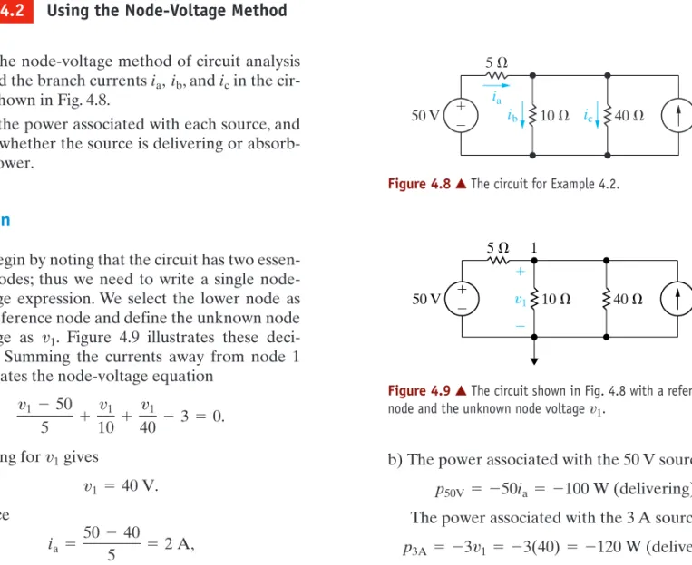
Using the Node-Voltage Method 94 4.3 Using the Node-Voltage Method with
Using the Mesh-Current Method 101 4.5 Using the Mesh-Current Method with
Understanding the Node-Voltage Method Versus Mesh-Current Method 107
Comparing the Node-Voltage and Mesh-Current Methods 108
Using Source Transformations to Solve a Circuit 110
Using Special Source Transformation Techniques 112
Finding the Thévenin Equivalent of a Circuit with a Dependent Source 116
Finding the Thévenin Equivalent Using a Test Source 118
Calculating the Condition for Maximum Power Transfer 121
Analyzing an Op Amp Circuit 149 5.2 Designing an Inverting Amplifier 151
Determining the Voltage, Given the Current, at the Terminals of an Inductor 177
Determining the Current, Given the Voltage, at the Terminals of an Inductor 178
Determining the Current, Voltage, Power, and Energy for an Inductor 180
Determining Current, Voltage, Power, and Energy for a Capacitor 184
Finding Mesh-Current Equations for a Circuit with Magnetically Coupled Coils 192
Determining the Natural Response of an RL Circuit 218
Determining the Natural Response of an RL Circuit with Parallel Inductors 219
Determining the Natural Response of an RC Circuit with Series Capacitors 223
Determining the Step Response of an RL Circuit 227
Determining the Step Response of an RC Circuit 230
Using the General Solution Method to Find an RC Circuit’s Step Response 233
Using the General Solution Method with Zero Initial Conditions 234
Using the General Solution Method to Find an RL Circuit’s Step Response 234
Determining the Step Response of a Circuit with Magnetically Coupled Coils 235
Analyzing an RC Circuit that has Sequential Switching 239
Finding the Unbounded Response in an RC Circuit 241
Finding the Roots of the Characteristic Equation of a Parallel RLC Circuit 269
Finding the Overdamped Natural Response of a Parallel RLC Circuit 272
Calculating Branch Currents in the Natural Response of a Parallel RLC Circuit 273
Finding the Underdamped Natural Response of a Parallel RLC Circuit 275
Finding the Critically Damped Natural Response of a Parallel RLC Circuit 278
Finding the Underdamped Step Response of a Parallel RLC Circuit 283
Finding the Critically Damped Step Response of a Parallel RLC Circuit 283
Comparing the Three-Step Response Forms 284 8.10 Finding Step Response of a Parallel RLC Circuit
Finding the Underdamped Natural Response of a Series RLC Circuit 287
Finding the Underdamped Step Response of a Series RLC Circuit 288
Analyzing Two Cascaded Integrating Amplifiers 290
Analyzing Two Cascaded Integrating Amplifiers with Feedback Resistors 293
Finding the Characteristics of a Sinusoidal Current 307
Finding the Characteristics of a Sinusoidal Voltage 308
Translating a Sine Expression to a Cosine Expression 308
Calculating the rms Value of a Triangular Waveform 308
Adding Cosines Using Phasors 314 9.6 Combining Impedances in Series 321
Using a Delta-to-Wye Transform in the Frequency Domain 325
Performing Source Transformations in the Frequency Domain 327
Finding a Thévenin Equivalent in the Frequency Domain 328
Using the Node-Voltage Method in the Frequency Domain 330
Using the Mesh-Current Method in the Frequency Domain 331
Analyzing a Linear Transformer in the Frequency Domain 335
Analyzing an Ideal Transformer Circuit in the Frequency Domain 340
Using Phasor Diagrams to Analyze a Circuit 342
Using Phasor Diagrams to Analyze Capacitive Loading Effects 343
Determining Average Power Delivered to a Resistor by Sinusoidal Voltage 367
Determining Maximum Power Transfer without Load Restrictions 378
Determining Maximum Power Transfer with Load Impedance Restriction 379
Finding Maximum Power Transfer with Impedance Angle Restrictions 380
Finding Maximum Power Transfer in a Circuit with an Ideal Transformer 381
Calculating Power in a Three-Phase Wye-Wye Circuit 411
Calculating Power in a Three-Phase Wye-Delta Circuit 411
Calculating Three-Phase Power with an Unspecified Load 412
Computing Wattmeter Readings in Three-Phase Circuits 415
Using Step Functions to Represent a Function of Finite Duration 430
Using the Convolution Integral to Find an Output Signal 491
Using the Transfer Function to Find
Designing a Series RC Low-Pass Filter 528 14.3 Designing a Series RL High-Pass Filter 532
Designing a Parallel RLC Bandpass Filter 539 14.7 Determining Effect of a Nonideal Voltage
Designing a Series RLC Bandreject Filter 546
Scaling a Prototype Low-Pass Op Amp Filter 563
Designing a Broadband Bandpass Op Amp Filter 567
Designing a Broadband Bandreject Op Amp Filter 570
Designing a Fourth-Order Low-Pass Op Amp Filter 574
Calculating Butterworth Transfer Functions 577
Designing a Fourth-Order Low-Pass Butterworth Filter 579
Determining the Order of a Butterworth Filter 582
An Alternate Approach to Determining the Order of a Butterworth Filter 582
Finding the Fourier Series of a Triangular Waveform with No Symmetry 607
Finding the Fourier Series of an Odd Function with Symmetry 614
Calculating Forms of the Trigonometric Fourier Series for Periodic Voltage 616
Calculating Average Power for a Circuit with a Periodic Voltage Source 623
Finding the Exponential Form of the Fourier Series 627
Using the Fourier Transform to Find the Transient Response 660
Using the Fourier Transform to Find the Sinusoidal Steady-State Response 661
Applying Parseval’s Theorem to a Low-Pass Filter 666
Finding the z Parameters of a Two-Port Circuit 679
Finding the a Parameters from Measurements 681
Finding h Parameters from Measurements and Table 18.1 684
WHY THIS EDITION?
In this text, we include numerous examples that present problem-solving techniques, followed by Assessment Problems that allow students to test their mastery of the material and techniques introduced. Students who would benefit from additional examples and practice problems can use the Student Workbook, which has been revised to reflect changes to the tenth edition of the text.
HALLMARK FEATURES
Each practical perspective problem is at least partially solved at the end of the chapter, and additional end-of-chapter problems may be assigned to allow students to further explore the practical perspective topic. Each manual presents the simulation material in the same order as the material is presented in the text.
Chapter Problems
Both students and instructors want to know how the generalized techniques presented in a first-year circuit analysis course relate to problems faced by practicing engineers. These manuals continue to include examples of circuits to be simulated that are taken directly from the text.
Practical Perspectives
Assessment Problems
Fundamental Equations and Concepts
Integration of Computer Tools
Design Emphasis
Accuracy
RESOURCES FOR STUDENTS
RESOURCES FOR INSTRUCTORS
PREREQUISITES
COURSE OPTIONS
ACKNOWLEDGMENTS
We are very grateful to the many teachers and students who have formally reviewed the text or more informally provided positive feedback and suggestions for improvement. We are privileged to have the opportunity to influence the educational experience of the many thousands of future engineers who will use this text.
ELECTRIC CIRCUITS
TENTH EDITION
Electrical Engineering: An Overview
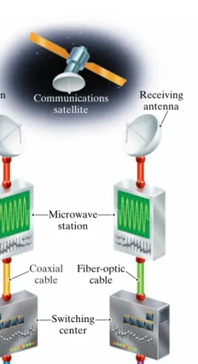
Starting at the left of the picture, inside a telephone, a microphone converts sound waves into electrical signals. A good example of interaction between systems is a commercial airplane, such as the one shown in Fig.

Circuit Theory
A good rule of thumb is: If the dimension of the system is (or smaller than) the dimension of the wavelength, you have a system with lumped parameters. Thus, as long as the physical dimension of the power system is less than m, we can treat it as a lumped-parameter system.
Problem Solving
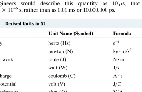
The International System of Units
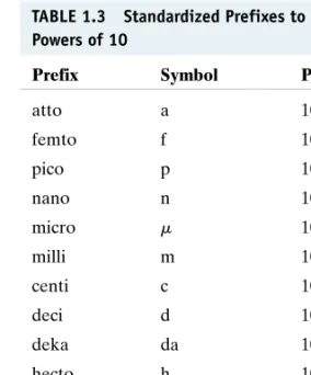
Standard prefixes corresponding to powers of 10, as given in Table 1.3, are then applied to the base unit. Example 1.1 Using SI units and prefixes for powers of 10 If a signal can travel in a cable at 80% of the speed of.

Solution
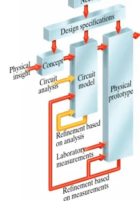
- Circuit Analysis: An Overview
- Voltage and Current
- The Ideal Basic Circuit Element
- Power and Energy
1.5 the voltage across the terminals of the box is indicated by , and the current in the circuit element is indicated by i. Objective 2 – Know and be able to use the definitions of voltage and current 1.3 The current at the terminals of the element i.
Balancing Power
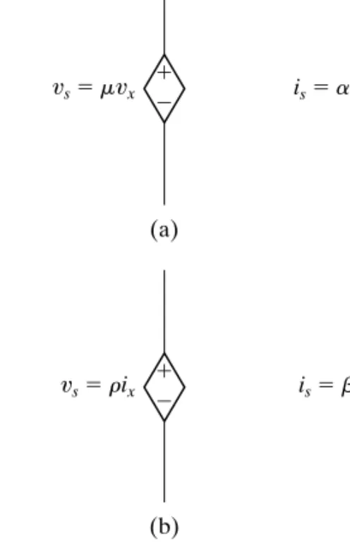
Voltage and Current Sources
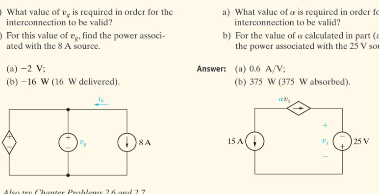
This requires each source to supply the same current in the same direction, which they do. The supply voltage of the independent source and the dependent source at the same pair of terminals, labeled a,b.
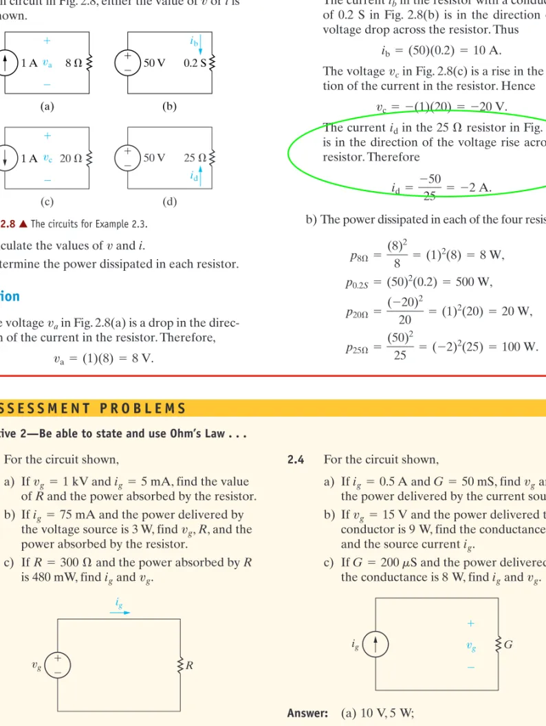
Electrical Resistance (Ohm’s Law)
A second method of expressing the power at the terminals of a resistor expresses power in terms of the current and the resistance. A third method of expressing the current at the terminals of a resistor is in terms of the voltage and resistance.
Construction of a Circuit Model
Starting with dry cell batteries, the positive terminal of the first cell is connected to the negative terminal of the second cell as shown in the figure. The positive terminal of the second cell is connected to one terminal of the lamp.

Kirchhoff’s Laws
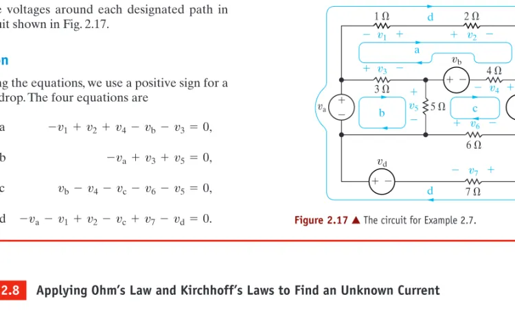
Example 2.6 Using Kirchhoff's Current Law Add the currents at each node in the circuit shown in Fig. Example 2.7 Using Kirchhoff's Voltage Law Sum the voltages around any given path in the circuit shown in Fig. 2.17.
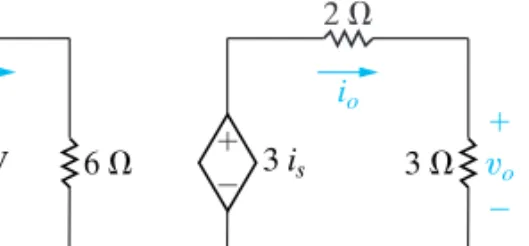
Analysis of a Circuit Containing Dependent Sources
There are three nodes in the circuit, so we turn to Kirchhoff's current law to generate the second equation. Example 2.10 illustrates another application of Ohm's law and Kirchhoff's laws to a dependent-source circuit.
Heating with Electric Radiators
Resistors in Series
The series connection in fig. 3.1) which says that if we know one of the seven streams, we know them all. Note that the resistance of the equivalent resistor is always greater than that of the largest resistor in the series connection.
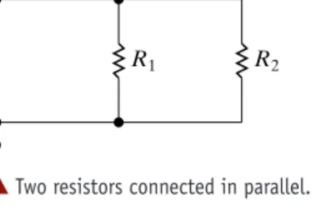
Resistors in Parallel
We therefore replace this series combination with a resistor, reducing the circuit to that shown in the figure. But is the voltage drop from node x to node y so we can go back to the circuit shown in the figure
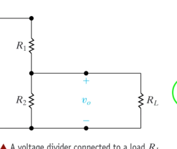
The Voltage-Divider
Another characteristic of the voltage divider circuit of interest is the sensitivity of the divider to the tolerances of the resistors. Example 3.2 Analysis of the voltage divider circuit The resistors used in the voltage divider circuit shown in fig.
The Current-Divider Circuit
- Voltage Division and Current Division
- Measuring Voltage and Current
- Measuring Resistance—
- Delta-to-Wye (Pi-to-Tee) Equivalent Circuits
To do this, we recognize that the equivalent resistance of the resistors connected in series is equal. By design, the deflection of the pointer is directly proportional to the current in the movable coil.
Resistive Touch Screens
Terminology
To discuss the more involved methods of circuit analysis, we need to define a few basic terms. So far, all circuits presented have been planar circuits, that is, circuits that can be drawn on a plane without intersecting branches. A circuit drawn with intersecting branches is still considered planar if it can be redrawn without intersecting branches.
Describing a Circuit—The Vocabulary
The node-voltage method is applicable to both planar and non-planar circuits, while the mesh-current method is limited to planar circuits.
Simultaneous Equations—How Many?
Furthermore, there is no current in the single conductor, so any circuit consisting of disconnected parts can always be reduced to a connected circuit.
The Systematic Approach—An Illustration
Introduction to the Node-Voltage Method
Thus the current away from node 1 through the resistor and the current away from node 1 through the resistor The sum of the three currents leaving node 1 must equal zero; therefore, the node-voltage equation is derived at node 1. Use the node-voltage method of circuit analysis to find the branch currents , , and in the circuit shown in Fig. 4.8.
The Node-Voltage Method and Dependent Sources
Substituting this relationship into the node equation 2 simplifies the two node-tension equations. Use the node voltage method to find the power .. connected to each source in the circuit shown.
The Node-Voltage Method
In general, when you use the node-voltage method to solve circuits that have voltage sources connected directly between significant nodes, the number of unknown node voltages is reduced. We also introduce the current because we cannot express the current in the dependent voltage source branch as a function of the node voltages and .
The Concept of a Supernode
Each node on each side of the dependent voltage source looks attractive because, if chosen, one of the node voltages would be known to be either (left node is the reference) or (right node is the reference). We now express the current driving the dependent voltage source as a function of the junction voltages:
Node-Voltage Analysis of the Amplifier Circuit
Introduction to the Mesh-Current Method
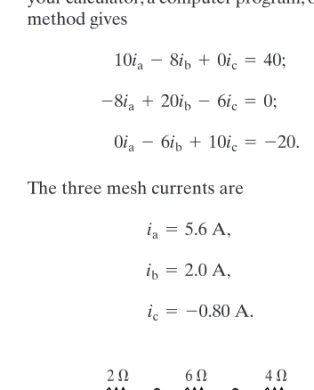
Thus, the mesh-current method is equivalent to a systematic substitution of the current equations into the voltage equations. Use the net current method to determine the power associated with each voltage source in the circuit shown in Fig. 4.21.
The Mesh-Current Method and Dependent Sources
Objective 2-Understand and be able to use the net current method 4.7 Use the net current method to find (a) the.
The Mesh-Current Method
The presence of the current source reduces the three unknown mesh currents to two such currents, because it limits the difference between and equal to 5 A. However, when we try to sum the voltages around mesh a or mesh c, we must insert into the equations the voltage of unknown in the 5 A current source.
The Concept of a Supermesh
Mesh-Current Analysis of the Amplifier Circuit
The Node-Voltage Method Versus the Mesh-Current Method
If so, using the nodal stress method will allow you to reduce the number of equations that need to be solved. Before proceeding, let's also review the circuit in terms of the node voltage method.
Source Transformations
For the circuit shown in fig. 4.37, find the power associated with the 6 V source. b) State whether the 6 V source absorbs or delivers the power calculated in (a). A current source in parallel with a resistor, as shown in fig. Example 4.9 Using special source transformation techniques.
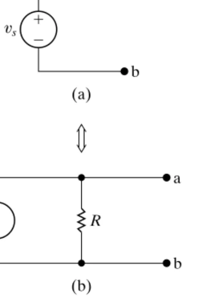
Thévenin and Norton Equivalents
If we place a short circuit across terminals a,b of the Thévenin equivalent circuit, the short circuit current directed from a to b is equal. The Thévenin resistance is therefore the ratio between the no-load voltage and the short-circuit current.
Finding a Thévenin Equivalent
Therefore, to calculate the Thévenin voltage, we simply calculate the open-circuit voltage of the original circuit. By hypothesis, this short-circuit current must be identical to the short-circuit current existing in a short-circuit placed across the terminals a,b of the original network.
The Norton Equivalent
4.45, the voltage across the resistor will be 24 V and the current in the resistor will be 1 A, as would be the case with the Thévenin circuit in Fig.
Using Source Transformations
More on Deriving a Thévenin Equivalent
If the circuit or network contains dependent sources, an alternative procedure for finding the Thévenin resistance is as follows. We first turn off the independent voltage source from the circuit and then excite the circuit from terminals a,b with either a test voltage source or a test current source.
Using the Thévenin Equivalent in the Amplifier Circuit
Maximum Power Transfer
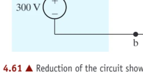
The maximum power transfer can best be described using the circuit shown in the figure. For the circuit shown in Figure 4.60, find the value that results in maximum power transfer.
Superposition
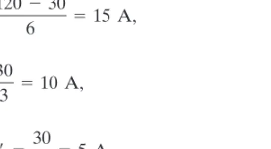
We demonstrate the superposition principle by using it to find the branch currents in the circuit shown in Figure 4.64. We determine the branch currents in the circuit shown in Figure 4.64 by first solving for the junction voltages across the 3 and the resistors respectively.
Circuits with Realistic Resistors
ÆLinear
The variable resistance ( ) in the circuit in Fig. P4.90 is adjusted for maximum power transfer to. The variable resistance in the circuit in Fig. P4.91 is adjusted for maximum power transfer to.
Operational Amplifier Terminals
This means that the terminals on each side of the package are in line and that the terminals on opposite sides of the package are also aligned. It is the reference terminal of the circuit in which the operational amplifier is built.
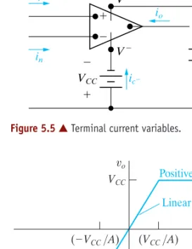
Terminal Voltages and Currents
So how do we know if an op amp is operating in its linear range. Note that the op amp is in its linear operating range because it lies between .
The Inverting-Amplifier Circuit
The result given by Eq. 5.10 is only valid if the operational amplifier shown in the circuit of fig. 5.9 is ideal; that is, if A is infinite and the input resistance is infinite. Because the inverting input current is almost zero, the voltage drop across is almost zero, and the inverting input voltage is almost equal to the signal voltage, that is, therefore, the op amp can only operate open loop in linear mode if if the op amp simply saturates.
The Summing-Amplifier Circuit
The Noninverting-Amplifier Circuit
Objective 2-To be able to analyze simple circuits containing ideal opamp-amps 5.4 Suppose that the opamp in the circuit shown . it is ideal. a) Find the output voltage when the variable resistor is set to . Thus, if we use the power supply for the non-inverting amplifier designed in part (a) and , the op amp will remain in its linear operating region.
The Difference-Amplifier Circuit
The Difference Amplifier—Another Perspective
Thus, an ideal difference amplifier amplified only the differential mode portion of the input voltage, eliminating the common mode portion of the input voltage. The noise appears as the common mode portion of the measured voltage, while the heartbeat voltages constitute the differential mode portion.
Measuring Difference-Amplifier Performance—
Thus, an ideal differential amplifier would amplify only the desired voltage and suppress the noise.
The Common Mode Rejection Ratio
A More Realistic Model for the Operational Amplifier
Such a model includes three modifications to the ideal op-amplifier: (1) a finite input resistance, (2) a finite open-loop gain,A; and (3) a non-zero output resistance, The circuit shown in Fig. To illustrate, we analyze both an inverting and a non-inverting amplifier, using the equivalent circuit shown in Fig.
Analysis of an Inverting-Amplifier Circuit Using the More Realistic Op Amp Model
Analysis of a Noninverting-Amplifier Circuit Using the More Realistic Op Amp Model
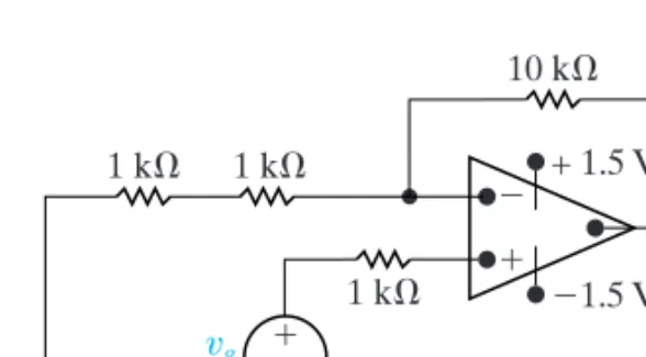
Objective 3—Understand the most realistic design for an operational amplifier 5.6 The inverting amplifier in the circuit shown has .. an input resistance of an output resistance and an open-loop gain of 300,000. Assume the amplifier is operating in its linear region. a) Calculate the voltage gain ( ) of the amplifier.
Strain Gages
The Inductor