CELLULAR WIRELESS NETWORKS

(1)

413 413

CHAPTER

C ELLULAR W IRELESS N ETWORKS

14.1 Principles of Cellular Networks 14.2 First-Generation Analog 14.3 Second-Generation CDMA 14.4 Third-Generation Systems

14.5 Recommended Reading and Web Sites 14.6 Key Terms, Review Questions, and Problems

413

14

(2)

After the fire of 1805, Judge Woodward was the central figure involved in reestab- lishing the town. Influenced by Major Pierre L’Enfant’s plans for Washington, DC, Judge Woodward envisioned a modern series of hexagons with major diagonal avenues centered on circular parks, or circuses, in the center of the hexagons. Fred- erick Law Olmstead said, ”nearly all of the most serious mistakes of Detroit’s past have arisen from a disregard of the spirit of Woodward’s plan.”

—Endangered Detroit, Friends of the Book-Cadillac Hotel

KEY POINTS

• The essence of a cellular network is the use of multiple low-power transmitters. The area to be covered is divided into cells in a hexagonal tile pattern that provide full coverage of the area.

• A major technical problem for cellular networks is fading, which refers to the time variation of received signal power caused by changes in the transmission medium or path(s).

• First-generation cellular networks were analog, making use of frequency division multiplexing.

• Second-generation cellular networks are digital. One technique in widespread use is based on code division multiple access (CDMA).

• The objective of the third-generation (3G) of wireless communication is to provide fairly high-speed wireless communications to support multimedia, data, and video in addition to voice.

Of all the tremendous advances in data communications and telecommunications, perhaps the most revolutionary is the development of cellular networks.

Cellular technology is the foundation of mobile wireless communications and supports users in locations that are not easily served by wired networks. Cellu- lar technology is the underlying technology for mobile telephones, personal communications systems, wireless Internet and wireless Web applications, and much more.

We begin this chapter with a look at the basic principles used in all cellular networks. Then we look at specific cellular technologies and standards, which are conveniently grouped into three generations. The first generation is analog based and, while still widely used, is passing from the scene. The dominant technology today is the digital second-generation systems. Finally, third-generation high- speed digital systems have begun to emerge.

(3)

d

R

d

dd dd

d

d d d 1.414

d

1.414 1.414 d

d

1.414 d

(a) Square pattern (b) Hexagonal pattern Figure 14.1 Cellular Geometries

14.1 PRINCIPLES OF CELLULAR NETWORKS

Cellular radio is a technique that was developed to increase the capacity available for mobile radio telephone service. Prior to the introduction of cellular radio, mobile radio telephone service was only provided by a high-power transmitter/receiver. A typical system would support about 25 channels with an effective radius of about 80 km. The way to increase the capacity of the system is to use lower-power systems with shorter radius and to use numerous transmitters/receivers. We begin this section with a look at the organization of cellular systems and then examine some of the details of their implementation.

Cellular Network Organization

The essence of a cellular network is the use of multiple low-power transmitters, on the order of 100 W or less. Because the range of such a transmitter is small, an area can be divided into cells, each one served by its own antenna. Each cell is allocated a band of frequencies and is served by a base station, consisting of transmitter, receiver, and control unit. Adjacent cells are assigned different frequencies to avoid interference or crosstalk. However, cells sufficiently distant from each other can use the same frequency band.

The first design decision to make is the shape of cells to cover an area. A matrix of square cells would be the simplest layout to define (Figure 14.1a).

However, this geometry is not ideal. If the width of a square cell is d, then a cell has four neighbors at a distance d and four neighbors at a distance As a mobile user within a cell moves toward the cell’s boundaries, it is best if all of the adjacent antennas are equidistant. This simplifies the task of determining when to switch the user to an adjacent antenna and which antenna to choose. A hexagonal pattern provides for equidistant antennas (Figure 14.1b). The radius of a hexagon is defined to be the radius of the circle that circumscribes it (equivalently, the distance from the center to each vertex; also equal to the length of a side of a

22d.

(4)

(c) Black cells indicate a frequency reuse for N 19

(a) Frequency reuse pattern for N 4 (b) Frequency reuse pattern for N 7 5 4

6 3 7 1

2

5 4 6

3 7

1 2

5 4 6

3 7

1 2 5 4 6

3 7 1

26 5 4 3 7

1 2

5 4 6

3 7 1

2

5 4 6

3 7 1

2

1 2 1

3 4 2 4

3 1 3

4 2 1 3 4 2 1 3 4 2

1 3 4 2

1 3 4 2 Circle with

radiusD

Figure 14.2 Frequency Reuse Patterns

hexagon). For a cell radius R, the distance between the cell center and each adjacent cell center is

In practice, a precise hexagonal pattern is not used. Variations from the ideal are due to topographical limitations, local signal propagation conditions, and practical limitation on siting antennas.

A wireless cellular system limits the opportunity to use the same frequency for different communications because the signals, not being constrained, can interfere with one another even if geographically separated. Systems supporting a large number of communications simultaneously need mechanisms to conserve spectrum.

Frequency Reuse

In a cellular system, each cell has a base transceiver. The transmission power is carefully controlled (to the extent that it is possible in the highly variable mobile communication environment) to allow communication within the cell using a given frequency while limiting the power at that frequency that escapes the cell into adjacent ones. The objective is to use the same frequency in other nearby cells, thus allowing the frequency to be used for multiple simultaneous conversations. Gen- erally, 10 to 50 frequencies are assigned to each cell, depending on the traffic expected.

The essential issue is to determine how many cells must intervene between two cells using the same frequency so that the two cells do not interfere with each other.

Various patterns of frequency reuse are possible. Figure 14.2 shows some examples. If d = 23R.

(5)

the pattern consists of Ncells and each cell is assigned the same number of frequencies, each cell can have K/Nfrequencies, where Kis the total number of frequencies allotted to the system. For AMPS (Section 14.2), and is the smallest pattern that can provide sufficient isolation between two uses of the same frequency.

This implies that there can be at most 57 frequencies per cell on average.

In characterizing frequency reuse, the following parameters are commonly used:

D=minimum distance between centers of cells that use the same band of frequencies (called cochannels)

R=radius of a cell

d=distance between centers of adjacent cells

N=number of cells in a repetitious pattern (each cell in the pattern uses a unique band of frequencies), termed the reuse factor

In a hexagonal cell pattern, only the following values of Nare possible:

Hence, possible values of Nare 1, 3, 4, 7, 9, 12, 13, 16, 19, 21, and so on. The following relationship holds:

This can also be expressed as

Increasing Capacity

In time, as more customers use the system, traffic may build up so that there are not enough frequencies assigned to a cell to handle its calls.A number of approaches have been used to cope with this situation, including the following:

• Adding new channels:Typically, when a system is set up in a region, not all of the channels are used, and growth and expansion can be managed in an orderly fashion by adding new channels.

• Frequency borrowing:In the simplest case, frequencies are taken from adjacent cells by congested cells.The frequencies can also be assigned to cells dynamically.

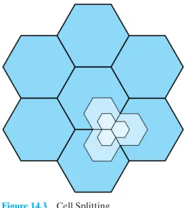
• Cell splitting:In practice, the distribution of traffic and topographic features is not uniform, and this presents opportunities for capacity increase. Cells in areas of high usage can be split into smaller cells. Generally, the original cells are about 6.5 to 13 km in size. The smaller cells can themselves be split; however, 1.5-km cells are close to the practical minimum size as a general solution (but see the subsequent discussion of microcells). To use a smaller cell, the power level used must be reduced to keep the signal within the cell. Also, as the mobile units move, they pass from cell to cell, which requires transferring of the call from one base transceiver to another. This process is called a handoff. As the cells get smaller, these handoffs become much more frequent.

Figure 14.3 indicates schematically how cells can be divided to provide more capacity. A radius reduction by a factor of Freduces the coverage area and increases the required number of base stations by a factor of F².

D/d = 2N.

D

R = 23N

N = I² + J² + 1I * J2, I,J = 0, 1, 2, 3,Á (d = 23R)

N = 7 K = 395,

(6)

Figure 14.3 Cell Splitting

Table 14.1 Typical Parameters for Macrocells and Microcells [ANDE95]

Macrocell Microcell

Cell radius 1 to 20 km 0.1 to 1 km

Transmission power 1 to 10 W 0.1 to 1 W

Average delay spread 0.1 to 10 to 100 ns

Maximum bit rate 0.3 Mbps 1 Mbps

10ms

• Cell sectoring:With cell sectoring, a cell is divided into a number of wedge- shaped sectors, each with its own set of channels, typically three or six sectors per cell. Each sector is assigned a separate subset of the cell’s channels, and directional antennas at the base station are used to focus on each sector.

• Microcells: As cells become smaller, antennas move from the tops of tall buildings or hills, to the tops of small buildings or the sides of large buildings, and finally to lamp posts, where they form microcells. Each decrease in cell size is accompanied by a reduction in the radiated power levels from the base stations and the mobile units. Microcells are useful in city streets in congested areas, along highways, and inside large public buildings.

Table 14.1 suggests typical parameters for traditional cells, called macrocells, and microcells with current technology.The average delay spread refers to multipath delay spread (i.e., the same signal follows different paths and there is a time delay between the earliest and latest arrival of the signal at the receiver). As indicated, the use of smaller cells enables the use of lower power and provides superior propagation conditions.

(7)

(b) Cell radius 0.8 km (a) Cell radius 1.6 km

Width 21 0.8 16.8 km Width 11 1.6 17.6 km

Height5兹31.613.9km Height10兹30.813.9km

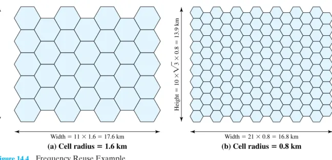
Figure 14.4 Frequency Reuse Example

EXAMPLE [HAAS00]. Assume a system of 32 cells with a cell radius of 1.6 km, a total of 32 cells, a total frequency bandwidth that supports 336 traffic channels, and a reuse factor of If there are 32 total cells, what geographic area is covered, how many channels are there per cell, and what is the total number of con- current calls that can be handled? Repeat for a cell radius of 0.8 km and 128 cells.

Figure 14.4a shows an approximately square pattern. The area of a hexagon of radius Ris A hexagon of radius 1.6 km has an area of and

the total area covered is For the number of chan-

nels per cell is for a total channel capacity of channels. For the layout of Figure 14.4b, the area covered is

The number of channels per cell is for a total channel capacity of channels.

48 * 128 = 6144

336/7 = 48,

1.66 * 128 = 213 km². 48 * 32 = 1536 336/7 = 48,

N = 7, 6.65 * 32 = 213 km².

6.65 km², 1.5R²23.

N = 7.

Operation of Cellular Systems

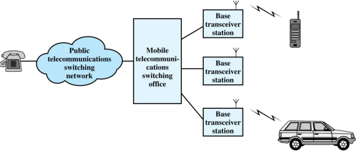
Figure 14.5 shows the principal elements of a cellular system. In the approximate center of each cell is a base station (BS). The BS includes an antenna, a controller, and a number of transceivers, for communicating on the channels assigned to that cell. The controller is used to handle the call process between the mobile unit and the rest of the network. At any time, a number of mobile user units may be active and moving about within a cell, communicating with the BS. Each BS is connected to a mobile telecommunications switching office (MTSO), with one MTSO serving multiple BSs. Typically, the link between an MTSO and a BS is by a wire line, although a wireless link is also possible. The MTSO connects calls between mobile units. The MTSO is also connected to the public telephone or telecommunications network and can make a connection between a fixed subscriber to the public network and a mobile subscriber to the cellular network. The MTSO assigns the voice channel to each call, performs handoffs, and monitors the call for billing information.

(8)

Base transceiver

station

station Mobile

telecommuni- cations switching

office Public

telecommunications switching

network

station

Figure 14.5 Overview of Cellular System

1Usually, but not always, the antenna and therefore the base station selected is the closest one to the mobile unit. However, because of propagation anomalies, this is not always the case.

The use of a cellular system is fully automated and requires no action on the part of the user other than placing or answering a call. Two types of channels are available between the mobile unit and the base station (BS): control channels and traffic channels.Control channelsare used to exchange information having to do with setting up and maintaining calls and with establishing a relationship between a mobile unit and the nearest BS.Traffic channelscarry a voice or data connection between users. Figure 14.6 illustrates the steps in a typical call between two mobile users within an area controlled by a single MTSO:

• Mobile unit initialization: When the mobile unit is turned on, it scans and selects the strongest setup control channel used for this system (Figure 14.6a).

Cells with different frequency bands repetitively broadcast on different setup channels. The receiver selects the strongest setup channel and monitors that channel. The effect of this procedure is that the mobile unit has automatically selected the BS antenna of the cell within which it will operate.¹Then a handshake takes place between the mobile unit and the MTSO controlling this cell, through the BS in this cell. The handshake is used to identify the user and register its location. As long as the mobile unit is on, this scanning procedure is repeated periodically to account for the motion of the unit. If the unit enters a new cell, then a new BS is selected. In addition, the mobile unit is monitoring for pages, discussed subsequently.

• Mobile-originated call:A mobile unit originates a call by sending the number of the called unit on the preselected setup channel (Figure 14.6b). The receiver at the mobile unit first checks that the setup channel is idle by examining information in the forward (from the BS) channel. When an idle is detected, the mobile may transmit on the corresponding reverse (to BS) channel. The BS sends the request to the MTSO.

(9)

(a) Monitor for strongest signal (b) Request for connection M

T S O

(c) Paging (d) Call accepted

M T S O

(e) Ongoing call

M T S O

(f) Handoff

M T S O

Figure 14.6 Example of Mobile Cellular Call

• Paging: The MTSO then attempts to complete the connection to the called unit. The MTSO sends a paging message to certain BSs depending on the called mobile number (Figure 14.6c). Each BS transmits the paging signal on its own assigned setup channel.

• Call accepted:The called mobile unit recognizes its number on the setup channel being monitored and responds to that BS, which sends the response to the MTSO. The MTSO sets up a circuit between the calling and called BSs. At the same time, the MTSO selects an available traffic channel within each BS’s cell and notifies each BS, which in turn notifies its mobile unit (Figure 14.6d). The two mobile units tune to their respective assigned channels.

(10)

• Ongoing call: While the connection is maintained, the two mobile units exchange voice or data signals, going through their respective BSs and the MTSO (Figure 14.6e).

• Handoff :If a mobile unit moves out of range of one cell and into the range of another during a connection, the traffic channel has to change to one assigned to the BS in the new cell (Figure 14.6f). The system makes this change without either interrupting the call or alerting the user.

Other functions performed by the system but not illustrated in Figure 14.6 include the following:

• Call blocking:During the mobile-initiated call stage, if all the traffic channels assigned to the nearest BS are busy, then the mobile unit makes a preconfig- ured number of repeated attempts. After a certain number of failed tries, a busy tone is returned to the user.

• Call termination:When one of the two users hangs up, the MTSO is informed and the traffic channels at the two BSs are released.

• Call drop:During a connection, because of interference or weak signal spots in certain areas, if the BS cannot maintain the minimum required signal strength for a certain period of time, the traffic channel to the user is dropped and the MTSO is informed.

• Calls to/from fixed and remote mobile subscriber:The MTSO connects to the public switched telephone network. Thus, the MTSO can set up a connection between a mobile user in its area and a fixed subscriber via the telephone network. Further, the MTSO can connect to a remote MTSO via the telephone network or via dedicated lines and set up a connection between a mobile user in its area and a remote mobile user.

Mobile Radio Propagation Effects

Mobile radio communication introduces complexities not found in wire communication or in fixed wireless communication. Two general areas of concern are signal strength and signal propagation effects.

• Signal strength: The strength of the signal between the base station and the mobile unit must be strong enough to maintain signal quality at the receiver but no so strong as to create too much cochannel interference with channels in another cell using the same frequency band. Several complicating factors exist.

Human-made noise varies considerably, resulting in a variable noise level. For example, automobile ignition noise in the cellular frequency range is greater in the city than in a suburban area. Other signal sources vary from place to place.

The signal strength varies as a function of distance from the BS to a point within its cell. Moreover, the signal strength varies dynamically as the mobile unit moves.

• Fading:Even if signal strength is within an effective range, signal propagation effects may disrupt the signal and cause errors. Fading is discussed subsequently in this section.

In designing a cellular layout, the communications engineer must take account of these various propagation effects, the desired maximum transmit power level at the

(11)

base station and the mobile units, the typical height of the mobile unit antenna, and the available height of the BS antenna. These factors will determine the size of the individual cell. Unfortunately, as just described, the propagation effects are dynamic and difficult to predict. The best that can be done is to come up with a model based on empirical data and to apply that model to a given environment to develop guidelines for cell size. One of the most widely used models was developed by Okumura et al.

[OKUM68] and subsequently refined by Hata [HATA80]. The original was a detailed analysis of the Tokyo area and produced path loss information for an urban environment. Hata’s model is an empirical formulation that takes into account a variety of environments and conditions. For an urban environment, predicted path loss is

L_dB= 69.55+26.16 logf_c-13.82 logh_t-A(h_r)+(44.9- 6.55 logh_t) log d (14.1) where

For a small- or medium-sized city, the correction factor is given by

And for a large city it is given by

To estimate the path loss in a suburban area, the formula for urban path loss in Equation (14.1) is modified as

And for the path loss in open areas, the formula is modified as

The Okumura/Hata model is considered to be among the best in terms of accuracy in path loss prediction and provides a practical means of estimating path loss in a wide variety of situations [FREE97, RAPP97].

L_dB1open2 = L_dB1urban2 - 4.781logf_c2² - 18.7331logf_c2 - 40.98 L_dB1suburban2 = L_dB1urban2 - 2[log1f_c/282]² - 5.4 A1h_r2 = 3.2[log111.75h_r2]² - 4.97 dB for f_c Ú 300 MHz A1h_r2 = 8.29[log11.54h_r2]² - 1.1 dB for f_c … 300 MHz

A1h_r2 = 11.1 log f_c - 0.72h_r - 11.56 log f_c - 0.82 dB A1h_r2 = correction factor for mobile antenna height

d = propagation distance between antennas in km, from 1 to 20 km h_r = height of receiving antenna 1mobile station2 in m, from 1 to 10 m h_t = height of transmitting antenna 1base station2 in m, from 30 to 300 m

f_c = carrier frequency in MHz from 150 to 1500 MHz

EXAMPLE [FREE97]. Let and

Estimate the path loss for a medium-size city.

= 69.55 + 77.28 - 22.14 - 8.95 + 34.4 = 150.14 dB

L_dB = 69.55+26.16 log 900-13.82 log 40 -8.95 + 144.9 -6.55 log 402 log 10

= 12.75 - 3.8 = 8.95 dB

A1h_r2 = 11.1 log 900 - 0.725 - 11.56 log 900 - 0.82 dB 10 km.

d = h_r = 5 m,

h_t = 40 m, f_c = 900 MHz,

(12)

R

R D

S

Lamp post

Figure 14.7 Sketch of Three Important Propagation Mechanisms: Reflection (R), Scatter- ing (S), Diffraction (D) [ANDE95]

2On the other hand, the reflected signal has a longer path, which creates a phase shift due to delay relative to the unreflected signal. When this delay is equivalent to half a wavelength, the two signals are back in phase.

Fading in the Mobile Environment

Perhaps the most challenging technical problem facing communications systems engineers is fading in a mobile environment. The term fadingrefers to the time variation of received signal power caused by changes in the transmission medium or path(s). In a fixed environment, fading is affected by changes in atmospheric conditions, such as rainfall. But in a mobile environment, where one of the two antennas is moving relative to the other, the relative location of various obstacles changes over time, creating complex transmission effects.

Multipath Propagation

Three propagation mechanisms, illustrated in Figure 14.7, play a role.Reflectionoccurs when an electromagnetic signal encounters a surface that is large relative to the wavelength of the signal. For example, suppose a ground-reflected wave near the mobile unit is received. Because the ground-reflected wave has a 180°

phase shift after reflection, the ground wave and the line-of-sight (LOS) wave may tend to cancel, resulting in high signal loss.²Further, because the mobile antenna is lower than most human-made structures in the area, multipath interference occurs. These reflected waves may interfere constructively or destructively at the receiver.

(13)

Diffractionoccurs at the edge of an impenetrable body that is large compared to the wavelength of the radio wave. When a radio wave encounters such an edge, waves propagate in different directions with the edge as the source. Thus, signals can be received even when there is no unobstructed LOS from the transmitter.

If the size of an obstacle is on the order of the wavelength of the signal or less, scatteringoccurs. An incoming signal is scattered into several weaker outgoing signals. At typical cellular microwave frequencies, there are numerous objects, such as lamp posts and traffic signs, that can cause scattering. Thus, scattering effects are difficult to predict.

These three propagation effects influence system performance in various ways depending on local conditions and as the mobile unit moves within a cell. If a mobile unit has a clear LOS to the transmitter, then diffraction and scattering are generally minor effects, although reflection may have a significant impact. If there is no clear LOS, such as in an urban area at street level, then diffraction and scattering are the primary means of signal reception.

The Effects of Multipath Propagation

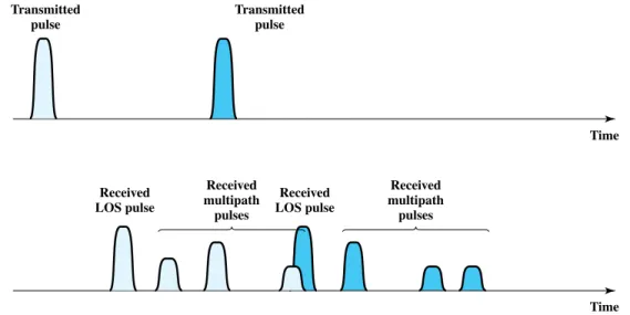
As just noted, one unwanted effect of multipath propagation is that multiple copies of a signal may arrive at different phases. If these phases add destructively, the signal level relative to noise declines, making signal detection at the receiver more difficult.

A second phenomenon, of particular importance for digital transmission, is intersymbol interference (ISI). Consider that we are sending a narrow pulse at a given frequency across a link between a fixed antenna and a mobile unit. Figure 14.8 shows what the channel may deliver to the receiver if the impulse is sent at two different times. The upper line shows two pulses at the time of transmission. The lower line shows the resulting pulses at the receiver. In each case the first received pulse is the desired LOS signal. The magnitude of that pulse may change because of changes in atmospheric attenuation. Further, as the mobile unit moves farther away from the fixed antenna, the amount of LOS attenuation increases. But in addition to this primary pulse, there may

Received LOS pulse

Received multipath pulses

Time Time Transmitted

pulse

Transmitted pulse

Received LOS pulse

Received multipath pulses

Figure 14.8 Two Pulses in Time-Variant Multipath

(14)

be multiple secondary pulses due to reflection, diffraction, and scattering. Now suppose that this pulse encodes one or more bits of data. In that case, one or more delayed copies of a pulse may arrive at the same time as the primary pulse for a subsequent bit.

These delayed pulses act as a form of noise to the subsequent primary pulse, making recovery of the bit information more difficult.

As the mobile antenna moves, the location of various obstacles changes; hence the number, magnitude, and timing of the secondary pulses change. This makes it difficult to design signal processing techniques that will filter out multipath effects so that the intended signal is recovered with fidelity.

Types of Fading

Fading effects in a mobile environment can be classified as either fast or slow. Referring to Figure 14.7, as the mobile unit moves down a street in an urban environment, rapid variations in signal strength occur over distances of about one-half a wavelength. At a frequency of 900 MHz, which is typical for mobile cellular applications, a wavelength is 0.33 m. Changes of amplitude can be as much as 20 or 30 dB over a short distance. This type of rapidly changing fading phenomenon, known as fast fading, affects not only mobile phones in automobiles, but even a mobile phone user walking down an urban street.

As the mobile user covers distances well in excess of a wavelength, the urban environment changes, as the user passes buildings of different heights, vacant lots, intersec- tions, and so forth. Over these longer distances, there is a change in the average received power level about which the rapid fluctuations occur. This is referred to as slow fading.

Fading effects can also be classified as flat or selective.Flat fading, or nonselective fading, is that type of fading in which all frequency components of the received signal fluctuate in the same proportions simultaneously.Selective fadingaffects unequally the different spectral components of a radio signal. The term selective fadingis usually significant only relative to the bandwidth of the overall communications channel. If attenuation occurs over a portion of the bandwidth of the signal, the fading is considered to be selective; nonselective fading implies that the signal bandwidth of interest is narrower than, and completely covered by, the spectrum affected by the fading.

Error Compensation Mechanisms

The efforts to compensate for the errors and distortions introduced by multipath fading fall into three general categories:

forward error correction, adaptive equalization, and diversity techniques. In the typical mobile wireless environment, techniques from all three categories are combined to combat the error rates encountered.

Forward error correction is applicable in digital transmission applications:

those in which the transmitted signal carries digital data or digitized voice or video data. Typically in mobile wireless applications, the ratio of total bits sent to data bits sent is between 2 and 3. This may seem an extravagant amount of overhead, in that the capacity of the system is cut to one-half or one-third of its potential, but the mobile wireless environment is so difficult that such levels of redundancy are necessary.

Chapter 6 discusses forward error correction.

Adaptive equalizationcan be applied to transmissions that carry analog information (e.g., analog voice or video) or digital information (e.g., digital data, digitized voice or video) and is used to combat intersymbol interference. The process of equalization involves some method of gathering the dispersed symbol energy back together into its original time interval. Equalization is a broad topic; techniques

(15)

include the use of so-called lumped analog circuits as well as sophisticated digital signal processing algorithms.

Diversityis based on the fact that individual channels experience independent fading events. We can therefore compensate for error effects by providing multiple logical channels in some sense between transmitter and receiver and sending part of the signal over each channel. This technique does not eliminate errors but it does reduce the error rate, since we have spread the transmission out to avoid being sub- jected to the highest error rate that might occur. The other techniques (equalization, forward error correction) can then cope with the reduced error rate.

Some diversity techniques involve the physical transmission path and are referred to as space diversity. For example, multiple nearby antennas may be used to receive the message, with the signals combined in some fashion to reconstruct the most likely transmitted signal. Another example is the use of collocated multiple directional antennas, each oriented to a different reception angle with the incoming signals again combined to reconstitute the transmitted signal.

More commonly, the term diversityrefers to frequency diversity or time diversity techniques. With frequency diversity, the signal is spread out over a larger frequency bandwidth or carried on multiple frequency carriers. The most important example of this approach is spread spectrum, which is examined in Chapter 9.

14.2 FIRST-GENERATION ANALOG

The original cellular telephone networks provided analog traffic channels; these are now referred to as first-generation systems. Since the early 1980s the most common first-generation system in North America has been the Advanced Mobile Phone Service (AMPS) developed by AT&T. This approach is also common in South America, Australia, and China. Although gradually being replaced by second-generation systems, AMPS is still in common use. In this section, we provide an overview of AMPS.

Spectral Allocation

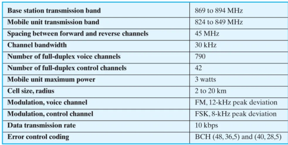
In North America, two 25-MHz bands are allocated to AMPS (Table 14.2), one for transmission from the base station to the mobile unit (869–894 MHz), the other for transmission from the mobile to the base station (824–849 MHz). Each of these bands is split in two to encourage competition (i.e., so that in each market two oper- ators can be accommodated). An operator is allocated only 12.5 MHz in each direc- tion for its system. The channels are spaced 30 kHz apart, which allows a total of 416 channels per operator. Twenty-one channels are allocated for control, leaving 395 to carry calls. The control channels are data channels operating at 10 kbps. The conversation channels carry the conversations in analog using frequency modulation. Con- trol information is also sent on the conversation channels in bursts as data. This number of channels is inadequate for most major markets, so some way must be found either to use less bandwidth per conversation or to reuse frequencies. Both approaches have been taken in the various approaches to mobile telephony. For AMPS, frequency reuse is exploited.

(16)

Table 14.2 AMPS Parameters

Base station transmission band 869 to 894 MHz

Mobile unit transmission band 824 to 849 MHz

Spacing between forward and reverse channels 45 MHz

Channel bandwidth 30 kHz

Number of full-duplex voice channels 790 Number of full-duplex control channels 42

Mobile unit maximum power 3 watts

Cell size, radius 2 to 20 km

Modulation, voice channel FM, 12-kHz peak deviation

Modulation, control channel FSK, 8-kHz peak deviation

Data transmission rate 10 kbps

Error control coding BCH (48, 36,5) and (40, 28,5)

Operation

Each AMPS-capable cellular telephone includes a numeric assignment module(NAM) in read-only memory. The NAM contains the telephone number of the phone, which is assigned by the service provider, and the serial number of the phone, which is assigned by the manufacturer. When the phone is turned on, it transmits its serial number and phone number to the MTSO (Figure 14.5); the MTSO maintains a database with information about mobile units that have been reported stolen and uses serial number to lock out stolen units. The MTSO uses the phone number for billing purposes. If the phone is used in a remote city, the service is still billed to the user’s local service provider.

When a call is placed, the following sequence of events occurs [COUC01]:

1. The subscriber initiates a call by keying in the telephone number of the called party and presses the send key.

2. The MTSO verifies that the telephone number is valid and that the user is autho- rized to place the call; some service providers require the user to enter a PIN (personal identification number) as well as the called number to counter theft.

3. The MTSO issues a message to the user’s cell phone indicating which traffic channels to use for sending and receiving.

4. The MTSO sends out a ringing signal to the called party. All of these operations (steps 2 through 4) occur within 10 s of initiating the call.

5. When the called party answers, the MTSO establishes a circuit between the two parties and initiates billing information.

6. When one party hangs up, the MTSO releases the circuit, frees the radio channels, and completes the billing information.

AMPS Control Channels

Each AMPS service includes 21 full-duplex 30-kHz control channels, consisting of 21 reverse control channels (RCCs) from subscriber to base station, and 21 forward

(17)

channels from base station to subscriber. These channels transmit digital data using FSK. In both channels, data are transmitted in frames.

Control information can be transmitted over a voice channel during a conversation. The mobile unit or the base station can insert a burst of data by turning off the voice FM transmission for about 100 ms and replacing it with an FSK-encoded message. These messages are used to exchange urgent messages, such as change power level and handoff.

14.3 SECOND-GENERATION CDMA

This section begins with an overview and then looks in detail at one type of second- generation cellular system.

First- and Second-Generation Cellular Systems

First-generation cellular networks, such as AMPS, quickly became highly popular, threatening to swamp available capacity. Second-generation systems have been developed to provide higher quality signals, higher data rates for support of digital services, and greater capacity. [BLAC99b] lists the following as the key differences between the two generations:

• Digital traffic channels: The most notable difference between the two generations is that first-generation systems are almost purely analog, whereas second-generation systems are digital. In particular, the first-generation systems are designed to support voice channels using FM; digital traffic is supported only by the use of a modem that converts the digital data into analog form. Second-generation systems provide digital traffic channels. These readily support digital data; voice traffic is first encoded in digital form before transmitting. Of course, for second-generation systems, the user traffic (data or digitized voice) must be converted to an analog signal for transmission between the mobile unit and the base station (e.g., see Figure 5.15).

• Encryption:Because all of the user traffic, as well as control traffic, is digitized in second-generation systems, it is a relatively simple matter to encrypt all of the traffic to prevent eavesdropping. All second-generation systems provide this capability, whereas first-generation systems send user traffic in the clear, providing no security.

• Error detection and correction:The digital traffic stream of second-generation systems also lends itself to the use of error detection and correction techniques, such as those discussed in Chapter 6. The result can be very clear voice reception.

• Channel access:In first-generation systems, each cell supports a number of channels. At any given time a channel is allocated to only one user. Second- generation systems also provide multiple channels per cell, but each channel is dynamically shared by a number of users using time division multiple access (TDMA) or code division multiple access (CDMA). We look at CDMA-based systems in this section.

(18)

3See Appendix J for a discussion of correlation and orthogonality.

Beginning around 1990, a number of different second-generation systems have been deployed. A good example is the IS-95 scheme using CDMA.

Code Division Multiple Access

CDMA for cellular systems can be described as follows. As with FDMA, each cell is allocated a frequency bandwidth, which is split into two parts, half for reverse (mobile unit to base station) and half for forward (base station to mobile unit). For full-duplex communication, a mobile unit uses both reverse and forward channels.

Transmission is in the form of direct-sequence spread spectrum (DS-SS), which uses a chipping code to increase the data rate of the transmission, resulting in an increased signal bandwidth. Multiple access is provided by assigning orthogonal chipping codes (defined in Chapter 9) to multiple users, so that the receiver can recover the transmission of an individual unit from multiple transmissions.

CDMA has a number of advantages for a cellular network:

• Frequency diversity: Because the transmission is spread out over a larger bandwidth, frequency-dependent transmission impairments, such as noise bursts and selective fading, have less effect on the signal.

• Multipath resistance:In addition to the ability of DS-SS to overcome multipath fading by frequency diversity, the chipping codes used for CDMA not only exhibit low cross correlation but also low autocorrelation.³ Therefore, a ver- sion of the signal that is delayed by more than one chip interval does not interfere with the dominant signal as much as in other multipath environments.

• Privacy:Because spread spectrum is obtained by the use of noiselike signals, where each user has a unique code, privacy is inherent.

• Graceful degradation: With FDMA or TDMA, a fixed number of users can access the system simultaneously. However, with CDMA, as more users access the system simultaneously, the noise level and hence the error rate increases; only gradually does the system degrade to the point of an unacceptable error rate.

Two drawbacks of CDMA cellular should also be mentioned:

• Self-jamming:Unless all of the mobile users are perfectly synchronized, the arriving transmissions from multiple users will not be perfectly aligned on chip boundaries. Thus the spreading sequences of the different users are not orthogonal and there is some level of cross correlation. This is distinct from either TDMA or FDMA, in which for reasonable time or frequency guard- bands, respectively, the received signals are orthogonal or nearly so.

• Near-far problem:Signals closer to the receiver are received with less attenuation than signals farther away. Given the lack of complete orthogonality, the transmissions from the more remote mobile units may be more difficult to recover.

Mobile Wireless CDMA Design Considerations

Before turning to the specific example of IS-95, it will be useful to consider some general design elements of a CDMA cellular system.

(19)

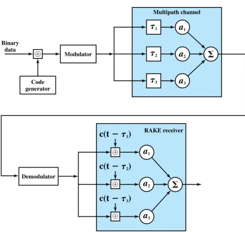
RAKE Receiver

In a multipath environment, which is common in cellular systems, if the multiple versions of a signal arrive more than one chip interval apart from each other, the receiver can recover the signal by correlating the chip sequence with the dominant incoming signal. The remaining signals are treated as noise. How- ever, even better performance can be achieved if the receiver attempts to recover the signals from multiple paths and then combine them, with suitable delays. This principle is used in the RAKE receiver.

Figure 14.9 illustrates the principle of the RAKE receiver. The original binary signal to be transmitted is spread by the exclusive-OR (XOR) operation with the transmitter’s chipping code. The spread sequence is then modulated for transmission over the wireless channel. Because of multipath effects, the channel generates multiple copies of the signal, each with a different amount of time delay ( etc.), and each with a different attenuation factors ( etc.).

At the receiver, the combined signal is demodulated. The demodulated chip stream is then fed into multiple correlators, each delayed by a different amount.

These signals are then combined using weighting factors estimated from the channel.

a₁,a₂, t1,t2,

Code generator Binary

data Modulator

Demodulator

Multipath channel

T

1

a

1

a

2

a

3

T

2

T

3

RAKE receiver

c(t T

1

)

c(t T

2

)

c(t T

3

)

a

1

a

2

a

3

Figure 14.9 Principle of RAKE Receiver [PRAS98]

(20)

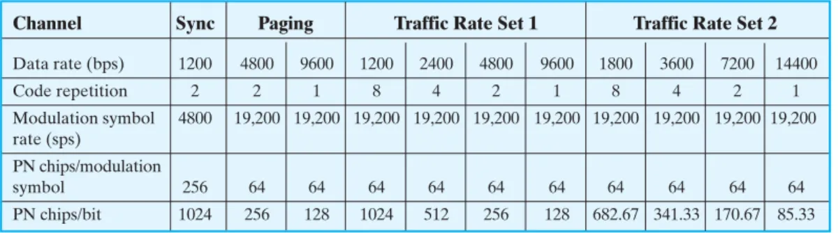
Table 14.3 IS-95 Forward Link Channel Parameters

Channel Sync Paging Traffic Rate Set 1 Traffic Rate Set 2

Data rate (bps) 1200 4800 9600 1200 2400 4800 9600 1800 3600 7200 14400

Code repetition 2 2 1 8 4 2 1 8 4 2 1

Modulation symbol 4800 19,200 19,200 19,200 19,200 19,200 19,200 19,200 19,200 19,200 19,200 rate (sps)

PN chips/modulation

symbol 256 64 64 64 64 64 64 64 64 64 64

PN chips/bit 1024 256 128 1024 512 256 128 682.67 341.33 170.67 85.33

IS-95

The most widely used second-generation CDMA scheme is IS-95, which is primarily deployed in North America. The transmission structures on the forward and reverse links differ and are described separately.

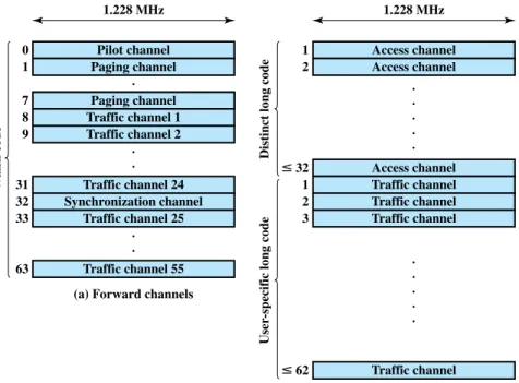
IS-95 Forward Link

Table 14.3 lists forward link channel parameters. The forward link consists of up to 64 logical CDMA channels each occupying the same 1228-kHz bandwidth (Figure 14.10a). The forward link supports four types of channels:

Pilot channel 1.228 MHz 0

1 7 8 9

31 32 33

63

Paging channel Paging channel Traffic channel 1 Traffic channel 2

Traffic channel 24 Synchronization channel

Traffic channel 25

Traffic channel 55 (a) Forward channels

Walshcode

Access channel 1.228 MHz 1

2

32 1 2 3

62

Access channel

Traffic channel Traffic channel Traffic channel

Traffic channel (b) Reverse channels

DistinctlongcodeUser-specificlongcode

Figure 14.10 IS-95 Channel Structure

(21)

• Pilot (channel 0): A continuous signal on a single channel. This channel allows the mobile unit to acquire timing information, provides phase refer- ence for the demodulation process, and provides a means for signal strength comparison for the purpose of handoff determination. The pilot channel consists of all zeros.

• Synchronization (channel 32):A 1200-bps channel used by the mobile station to obtain identification information about the cellular system (system time, long code state, protocol revision, etc.).

• Paging (channels 1 to 7):Contain messages for one or more mobile stations.

• Traffic (channels 8 to 31 and 33 to 63): The forward channel supports 55 traffic channels. The original specification supported data rates of up to 9600 bps. A subsequent revision added a second set of rates up to 14,400 bps.

Note that all of these channels use the same bandwidth. The chipping code is used to distinguish among the different channels. For the forward channel, the chipping codes are the 64 orthogonal 64-bit codes derived from a matrix known as the Walsh matrix (discussed in [STAL05]).

Figure 14.11 shows the processing steps for transmission on a forward traffic channel using rate set 1. For voice traffic, the speech is encoded at a data rate of 8550 bps. After additional bits are added for error detection, the rate is 9600 bps. The full channel capacity is not used when the user is not speaking. During quiet periods the data rate is lowered to as low as 1200 bps. The 2400-bps rate is used to transmit tran- sients in the background noise, and the 4800-bps rate is used to mix digitized speech and signaling data.

The data or digitized speech is transmitted in 20-ms blocks with forward error correction provided by a convolutional encoder with rate 1/2, thus doubling the effective data rate to a maximum of 19.2 kbps. For lower data rates, the encoder output bits (called code symbols) are replicated to yield the 19.2-kbps rate. The data are then interleaved in blocks to reduce the effects of errors by spreading them out.

Following the interleaver, the data bits are scrambled. The purpose of this is to serve as a privacy mask and to prevent the sending of repetitive patterns, which in turn reduces the probability of users sending at peak power at the same time. The scrambling is accomplished by means of a long code that is generated as a pseudorandom number from a 42-bit-long shift register. The shift register is initialized with the user’s electronic serial number. The output of the long code generator is at a rate of 1.2288 Mbps, which is 64 times the rate of 19.2 kbps, so only one bit in 64 is selected (by the decimator function). The resulting stream is XORed with the output of the block interleaver.

The next step in the processing inserts power control information in the traffic channel, to control the power output of the antenna. The power control function of the base station robs the traffic channel of bits at a rate of 800 bps. These are inserted by stealing code bits. The 800-bps channel carries information directing the mobile unit to increment, decrement, or keep stable its current output level. This power control stream is multiplexed into the 19.2 kbps by replacing some of the code bits, using the long code generator to encode the bits.

64 * 64

(22)

Add frame quality indica- tors for 9600 &

4800 bps rates 8.6 kbps 4.0 kbps 2.0 kbps 0.8 kbps

9.6 kbps 4.8 kbps 2.4 kbps 1.2 kbps

Code symbol

19.2 kbps

800 Hz 19.2 kbps

19.2 kbps

Code symbol

19.2 ksps

Code symbol

Add 8-bit encoder tail

Convolutional encoder (n,k,K) (2, 1, 9)

QPSK modulator Long code

generator Long code mask

for user m

Power control bits 800 bps

Transmitted signal PN chip 1.2288 Mbps 1.2288 Mbps

Walsh coden

Symbol repetition

Block interleaver Forward traffic channel

information bits (172, 80, 40, or 16 b/frame)

Decimator

Decimator Multiplexor

Figure 14.11 IS-95 Forward Link Transmission

The next step in the process is the DS-SS function, which spreads the 19.2 kbps to a rate of 1.2288 Mbps using one row of the Walsh matrix.

One row of the matrix is assigned to a mobile station during call setup. If a 0 bit is presented to the XOR function, then the 64 bits of the assigned row are sent.

If a 1 is presented, then the bitwise XOR of the row is sent. Thus, the final bit rate is 1.2288 Mbps. This digital bit stream is then modulated onto the carrier using a QPSK modulation scheme. Recall from Chapter 5 that QPSK involves creating two bit streams that are separately modulated (see Figure 5.11).

In the IS-95 scheme, the data are split into I and Q (in-phase and quadrature) channels and the data in each channel are XORed with a unique short code. The short codes are generated as pseudorandom numbers from a 15-bit-long shift register.

64 * 64

(23)

Table 14.4 IS-95 Reverse Link Channel Parameters

Channel Access Traffic-Rate Set 1 Traffic-Rate Set 2

Data rate (bps) 4800 1200 2400 4800 9600 1800 3600 7200 14400

Code rate 1/3 1/3 1/3 1/3 1/3 1/2 1/2 1/2 1/2

Symbol rate before 14,400 3600 7200 14,400 28,800 3600 7200 14,400 28,800 repetition (sps)

Symbol repetition 2 8 4 2 1 8 4 2 1

Symbol rate after 28,800 28,800 28,800 28,800 28,800 28,800 28,800 28,800 28,800 repetition (sps)

Transmit duty cycle 1 1/8 1/4 1/2 1 1/8 1/4 1/2 1

Code symbols/ 6 6 6 6 6 6 6 6 6

modulation symbol

PN chips/ 256 256 256 256 256 256 256 256 256

modulation symbol

PN chips/bit 256 128 128 128 128 256/3 256/3 256/3 256/3

IS-95 Reverse Link

Table 14.4 lists reverse link channel parameters. The reverse link consists of up to 94 logical CDMA channels each occupying the same 1228-kHz bandwidth (Figure 14.10b). The reverse link supports up to 32 access channels and up to 62 traffic channels.

The traffic channels in the reverse link are mobile unique. Each station has a unique long code mask based on its electronic serial number. The long code mask is a 42-bit number, so there are different masks. The access channel is used by a mobile to initiate a call, to respond to a paging channel message from the base station, and for a location update.

Figure 14.12 shows the processing steps for transmission on a reverse traffic channel using rate set 1. The first few steps are the same as for the forward channel. For the reverse channel, the convolutional encoder has a rate of 1/3, thus tripling the effective data rate to a maximum of 28.8 kbps. The data are then block interleaved.

The next step is a spreading of the data using the Walsh matrix. The way in which the matrix is used, and its purpose, are different from that of the forward channel. In the reverse channel, the data coming out of the block interleaver are grouped in units of 6 bits. Each 6-bit unit serves as an index to select a row of the Walsh matrix and that row is substituted for the input. Thus the data rate is expanded by a factor of 64/6 to 307.2 kbps. The purpose of this encoding is to improve reception at the base station. Because the 64 possible codings are orthogonal, the block coding enhances the decision-making algorithm at the receiver and is also computationally efficient (see [PETE95] for details). We can view this Walsh modulation as a form of block error-correcting code with

and In fact, all distances are 32.

The data burst randomizer is implemented to help reduce interference from other mobile stations (see [BLAC99b] for a discussion). The operation

d_min = 32.

1n,k2 = 164, 62

12⁶ = 642, 64 * 64

2⁴² - 1

(24)

Add frame quality indica- tors for 9600 &

4800 bps rates 8.6 kbps 4.0 kbps 2.0 kbps 0.8 kbps

Code symbol

28.8 ksps Code symbol

4.8 ksps (307.2 kcps)

Modulation symbol (Walsh chip) 9.2 kbps

4.4 kbps 2.0 kbps 0.8 kbps

Add 8-bit encoder tail

Convolutional encoder (n,k,K) (3, 1, 9)

64-ary orthogonal modulator

Data burst randomizer

OQPSK modulator Long code

generator

Long code mask

Transmitted signal PN chip 1.2288 Mbps

Symbol repetition

Block interleaver Reverse traffic channel

information bits (172, 80, 40, or 16 b/frame)

Figure 14.12 IS-95 Reverse Link Transmission

involves using the long code mask to smooth the data out over each 20-ms frame.

The next step in the process is the DS-SS function. In the case of the reverse channel, the long code unique to the mobile is XORed with the output of the randomizer to produce the 1.2288-Mbps final data stream. This digital bit stream is then modulated onto the carrier using an offset QPSK modulation scheme. This differs from the forward channel in the use of a delay element in the modulator (Figure 5.11) to produce orthogonality. The reason the modulators are different is that in the forward channel, the spreading codes are orthogonal, all coming from the Walsh matrix, whereas in the reverse channel, orthogonality of the spreading codes is not guaranteed.

(25)

14.4 THIRD-GENERATION SYSTEMS

The objective of the third generation (3G) of wireless communication is to provide fairly high-speed wireless communications to support multimedia, data, and video in addition to voice. The ITU’s International Mobile Telecommunications for the year 2000 (IMT-2000) initiative has defined the ITU’s view of third-generation capabili- ties as

• Voice quality comparable to the public switched telephone network

• 144-kbps data rate available to users in high-speed motor vehicles over large areas

• 384 kbps available to pedestrians standing or moving slowly over small areas

• Support (to be phased in) for 2.048 Mbps for office use

• Symmetrical and asymmetrical data transmission rates

• Support for both packet-switched and circuit-switched data services

• An adaptive interface to the Internet to reflect efficiently the common asym- metry between inbound and outbound traffic

• More efficient use of the available spectrum in general

• Support for a wide variety of mobile equipment

• Flexibility to allow the introduction of new services and technologies

More generally, one of the driving forces of modern communication technology is the trend toward universal personal telecommunications and universal communications access. The first concept refers to the ability of a person to identify himself or herself easily and use conveniently any communication system in an entire country, over a continent, or even globally, in terms of a single account. The second refers to the capability of using one’s terminal in a wide variety of environments to connect to information services (e.g., to have a portable terminal that will work in the office, on the street, and on airplanes equally well). This revolution in personal computing will obviously involve wireless communication in a fundamental way.

Personal communications services (PCSs) and personal communication networks (PCNs) are names attached to these concepts of global wireless communications, and they also form objectives for third-generation wireless.

Generally, the technology planned is digital using time division multiple access or code division multiple access to provide efficient use of the spectrum and high capacity.

PCS handsets are designed to be low power and relatively small and light.

Efforts are being made internationally to allow the same terminals to be used worldwide.

Alternative Interfaces

Figure 14.13 shows the alternative schemes that have been adopted as part of IMT-2000. The specification covers a set of radio interfaces for optimized performance

(26)

Radio interface

IMT-DS Direct spread

(W-CDMA)

IMT-MC Multicarrier

(cdma2000)

IMT-TC Time code (TD-CDMA)

IMT-SC Single carrier

(TDD)

IMT-FT Frequency-time

(DECT)

CDMA-based networks

TDMA-based networks

FDMA-based networks Figure 14.13 IMT-2000 Terrestrial Radio Interfaces

in different radio environments. A major reason for the inclusion of five alternatives was to enable a smooth evolution from existing first- and second-generation systems.

The five alternatives reflect the evolution from the second generation. Two of the specifications grow out of the work at the European Telecommunications Stan- dards Institute (ETSI) to develop a UMTS (universal mobile telecommunications system) as Europe’s 3G wireless standard. UMTS includes two standards. One of these is known as wideband CDMA, or W-CDMA. This scheme fully exploits CDMA technology to provide high data rates with efficient use of bandwidth.

Table 14.5 shows some of the key parameters of W-CDMA. The other European effort under UMTS is known as IMT-TC, or TD-CDMA. This approach is a combi- nation of W-CDMA and TDMA technology. IMT-TC is intended to provide an upgrade path for the TDMA-based GSM systems.

Another CDMA-based system, known as cdma2000, has a North American origin. This scheme is similar to, but incompatible with, W-CDMA, in part because the standards use different chip rates. Also, cdma2000 uses a technique known as multicarrier, not used with W-CDMA.

Two other interface specifications are shown in Figure 14.13. IMT-SC is primarily designed for TDMA-only networks. IMT-FT can be used by both TDMA and FDMA carriers to provide some 3G services; it is an outgrowth of the Digital Euro- pean Cordless Telecommunications (DECT) standard.