For their helpful discussions on a wide range of technical topics, my thanks to Arthur Sheeman, Bobby. Thanks to Sandy Weinreb for a very educational summer at NRAO and for his helpful discussions since.
Introduction
Historical Perspective
This package, known as 8409, allowed the calibration of systematic errors in the network analyzer. The sampled line network analyzer discussed in this thesis is an outgrowth of the six-port network analyzer.
Organization of the Thesis
Hoer, “Using six-port and eight-port junctions to measure active and passive circuit parameters,” Nat.
F'our-Port Network Analyzer Theory
Reflection Measurements with the 4-Port Network Analyzer
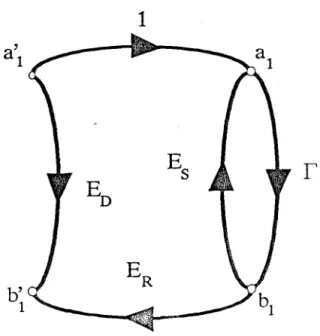
The final result is therefore that the value f' indicated on the vector voltmeter is a bilinear transformation of the actual value of r. Ev is the directional error related to the imperfect direction of the couplers in the test set.
S-Parameter Measurements with the 4-Port Network Analyzer
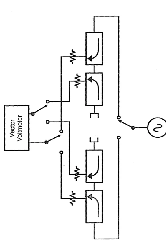
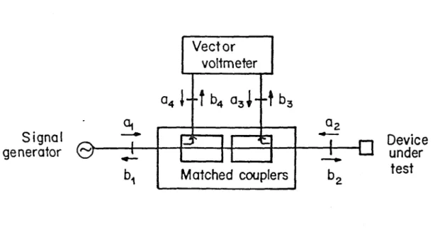
When performing a transmission measurement, terminal 2 of the device under test is connected directly to the vector voltmeter so that the meter measures b5/b4. Attenuators are placed between the four-port network and the vector voltmeter, and between port 2 of the device under test and the return port of the transmission, as shown in Figure 2.6.
Six-Port Network Analyzer Theory
Reflection Measurements with the 6-Port Network Analyzer
Among the calibration constants, a limiting relationship can be found based solely on the linearity of the six-port network. This layout specifies the specific six-port network used in the network analyzer implementation.
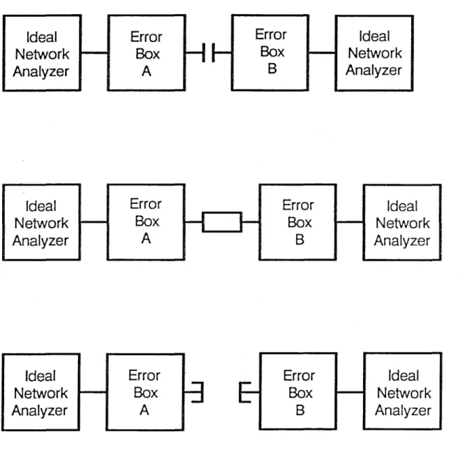
Dual Reflectometer Calibration - the TRL Scheme
The goal of the TRL calibration procedure is to determine the parameters of the error boxes A and B. The T parameters are defined by. 3.57) The T-matrix of the cascade of two networks is just the product of the T-matrices of the two networks. U that is observed is given by where L represents the T parameters of the line inserted between the two reflectometers.
An assumption must be made about the value of the L, T parameters for the length of line used as the calibration standard. Approximate knowledge of the properties of the line calibration standard can be used to answer this question.
S-Parameter Measurements with the 6-Port Network Analyzer
Most six-port reflectometers have their best accuracy when measuring values of r for which 1r1 < 1. Engen, "Calibration of an arbitrary six-port junction for measuring active and passive circuit parameters," IEEE Trans. Engen, “An improved circuit for implementing the six-port technique of microwave measurements,” IEEE Trans.
Hoer, "'Thru-reflect-line': An improved technique for calibrating the dual six-port automatic network analyzer," IEEE Trans. Hoer, “Calibration of two six-port reflectometers with an unknown precision transmission line length,” in 1978 IEEE MTT-S Int.
Sampled-Line Network Analyzer Theory
Placement of the Measurement Centers
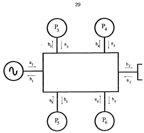
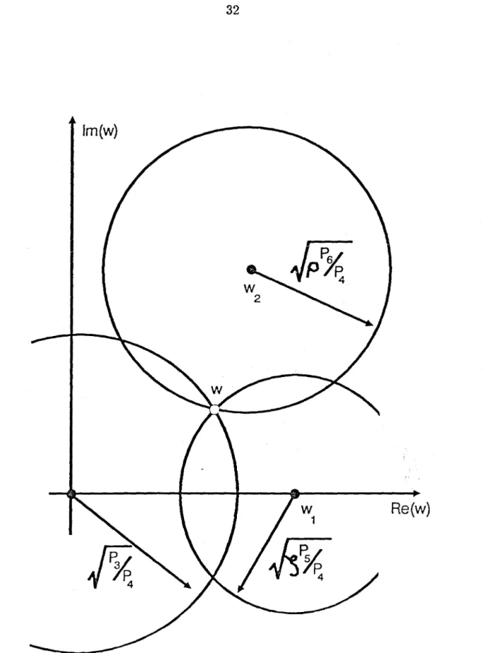
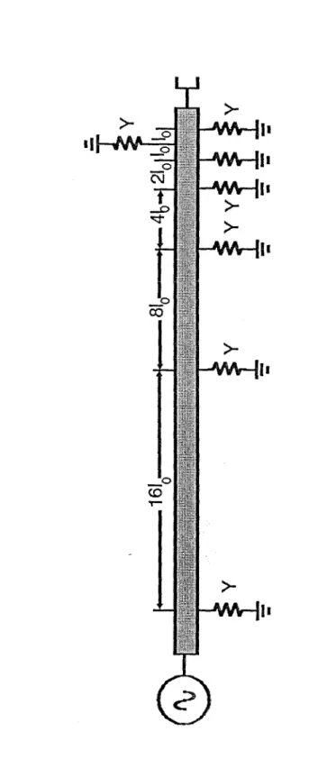
Given that the patterned line analyzer is a six-port type, the best way to examine its performance is to consider placing the measurement centers w1, w2 in the w plane. The B's are the electrical lengths of the various sections of the transmission line, and the detectors are numbered as shown. Their response is the square of the magnitude of the voltage at the connection point on the line.
It is interesting to note how the transformation process symmetrizes the error around the origin of the I'-plane. Experimentally, values in the range of 3 to 6 dB have been found to be satisfactory with various versions of the sampled line analyzer.

Calibration and Measurement Options
Here, Wi is the position of the ith measurement center, Ri is the distance from w to wi predicted by the measurement (Rr = (iPi/P4 ), and Ci is the weighting factor.
Effects of Detector Loading
The standing wave pattern for the matched load case now has a magnitude comparable to that of the short circuit. Here the detector admittance has increased to 0.2Y0 • The open circuit and matched load patterns are starting to look similar and the open circuit and short circuit phases are moving together. Here, the values of the measurement centers and the position and size of the transformed /fj = 1 circle in the w-plane are calculated for several detector admittance values.
For the GHz frequency range, the primary triplet for the analyzer consists of the first, second and seventh diodes numbered from the generator. The secondary triple given as an example consists of the first, second and third diodes.
The Elf Network Analyzer
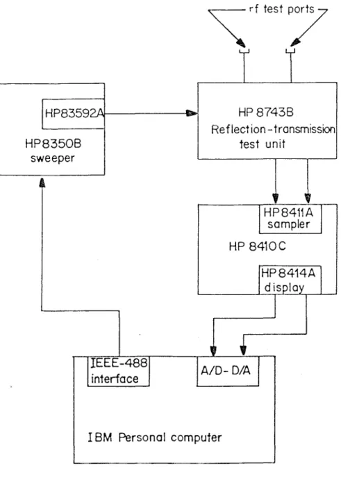
Hardware Description
The computer communicates with the rest of the system through two interface cards, a general purpose A/D and D/A card [1] and an IEEE-488 bus interface card [2]. In the configuration shown, the IEEE-488 card is used to set the frequency of the sweep oscillator, and the A/D card reads the value of the network analyzer measurement from the horizontal and vertical outputs of the HP 8414A polar display using be with the analyst. The vector voltmeter of the HP 8410B network analyzer is a phase-locked receiver, so it automatically follows the frequency of the sweep oscillator.
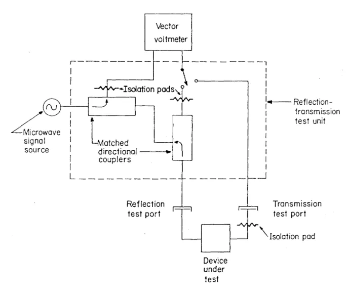
Attenuators and directional coupler isolation are used to reduce the effects of switches on the network, a requirement described in Chapter 2. determine the constants of the linear relationship between voltage and frequency.
Software Description
- Mode Selection, Calibration, and Measurement
- Manipulation, Storage and Display
The effect is to calibrate the resistance based on the characteristic impedance of the line into which the load slides, and not on the load itself. After selecting the measurement mode and returning to the mam menu, enter '3' to select the frequency range of the measurement. Selection five can then be used to choose a subrange of the source's frequency sweep.
With the 'Screen' option, the table of the selected S-parameter scrolls down SGreen in polar form. In practice, the data areas of the menu will show something other than zeros.

Sample Measurement
Saleh, “Explicit formulas for error correction in microwave measurement sets with switching-dependent port mismatches,” IEEE Trans. Sodomsky, “An explicit solution for the dispersion parameters of a linear two-port with an imperfect test set,” IEEE Trans.

The Sprite Sampled-Line Network Analyzer
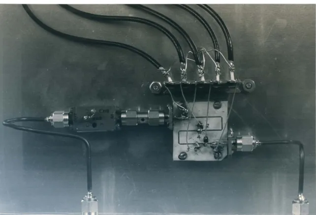
Hardware Description
The detector circuit used in the first analyzer provided good isolation of the detectors from the microstrip line. The additional loss observed in the sample line analyzer is attributed to the effects of the samplers on the line. The fourth analyzer appears to be the best implementation of the sampled line analyzer to date.
Turbo C was chosen as the compiler for the current version of the sampled-line network analyzer program. A secondary triple consists of the first two diodes in the primary triple, and a new third diode.
- The Microwave Phase Shifter
- The Preamplifier Bank
- The Synchronization Circuitry
Software Description
The same diode voltage, that of the first diode in all triples, is the denominator for all the ratios used in the calibration procedures. In the last phase of the calibration procedure, the Cs are found as described in Chapter 3, which allows the determination of a2f a1 from the observed reflection coefficients. This final calibration step uses data from the same five delay lines used in the TRL calibration.
However, instead of selecting one best line, as is necessary in the TRL process, data from all measurements of the delay lines are used to form a least-squares estimate of the C's. This makes examining the measured data easy, and viewing the calibration data is often helpful in diagnosing problems in the Sprite hardware.
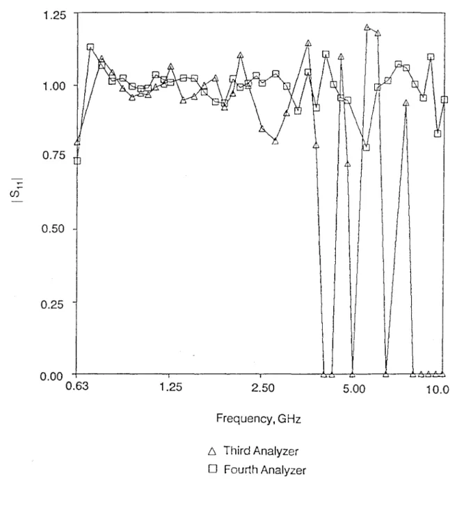
Sample Measurements
There is an error at the high end of the range, again probably due to a treble that is stretched too far in frequency. Over most of the first octave, the magnitude of the error vector in the fourth analyzer is about 0.02. In the second it increases to about 0.04 and is about 0.06 in the middle regions of the third and fourth octaves.
Due to the poor performance of the third sample line analyzer, which is used as one of the heads in the S-parameter measurement system, calibrations and measurements can only be performed reliably up to 3.5 GHz or more. Here again, the error in determining S22 is large because of the problem with the third reflectometer head.
Conclusions and Suggestions for Future Work
Thin Film Sampler Design
The chip components, particularly the resistors used in the present sampled-line analyzer, have parasitic capacitances too high to meet these requirements at frequencies well above 10 GHz. Aluminum oxide substrates are available with special metallizations that can be used to fabricate thin film resistors on the substrates through an etching process. The gold layer is etched away wherever a resistor is to be placed, exposing the TiW.
Since lines of 2 mils or less in width can be achieved with thin film etching techniques, resistive sampling circuits with very low parasitic capacitances can be fabricated this way. Sampling circuits constructed in this manner should be able to provide acceptable line loading and RF-DC isolation at least up to 20 GHz.
Monolithic Fabrication Options
The inductance for this structure could be implemented as a constriction of the microstrip line near the diode. This design would require some careful modeling, especially if the design is to extend into the millimeter wave region. In monolithic manufacturing it may also be desirable to use something other than microstrip for the sampled transmission line.
Planar transmission lines, such as coplanar waveguide, slot line, or coplanar strips, keep all waveguide conductors on the same side of the substrate, eliminating the need for vias to connect to the ground plate.

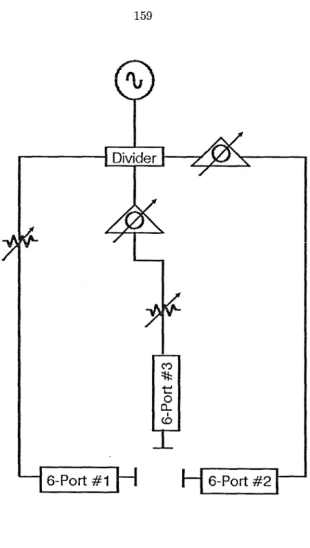
Measurement of Multi-Port Networks
If this ambiguity can be resolved by knowledge of the device under test, the S-parameter measurement is complete. For each combination of phase shifter positions in the system, a different set of these fourteen coefficients must be found and stored. The desired result is a set of expressions for the true S-parameters of the device under test in terms of the measured values and the six calibration constants.
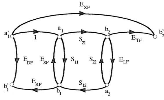
The starting point is equations (2.20) and (2.29), which give the measured values in terms of true values and constants. Two equations of the same form, resulting from the measurement in the reverse direction, complete the set.