Introduction
Thesis Organization
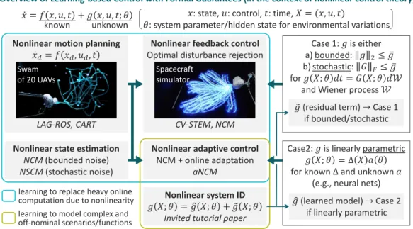
Overview of learning-based control with formal guarantees (in the context of nonlinear control theory). In Chapter 5, we derive several theorems that form the basis of learning-based control using contraction theory.
Related Work
A motivation for optimization-based approaches to the design of the contraction metric is suggested in that the Hamilton-Jacobi inequality for the L2 stability condition with finite gain can be expressed as LMI when the contraction theory is equipped with the extended linearity of the SDC formulation. . This means that contraction theory could be used as a central tool in realizing safe and robust operations on learning-based and data-driven control, estimation and motion planning schemes in real-world scenarios.

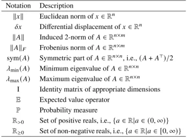
Notation
One of the distinguishing features of contraction theory in Theorem 2.1 is incremental stability with exponential convergence. Suppose that the systems (6.4) and (6.5) are estimated with an estimator gain𝐿𝐿, which calculates𝐿 from the CV-STEM estimator.
Contraction Theory
Fundamentals
Note that the smoothness of 𝑓(𝑥 , 𝑡) guarantees the existence and uniqueness of the solution of (2.1) for a given𝑥(0) =𝑥0 at least locally [9, p. - rem 2.2, let's consider the following closed-loop Lagrangian system [14, p.
Path-Length Integral and Robust Incremental Stability Analysis
Note that the shortest path integral𝑉ℓof(2.22)with a parameterized state𝑥(i.e.,inf𝑉ℓ =√ . inf𝑉𝑠ℓ) defines the Riemannian distance and the path integral of a minimizing geodesic [21]. As a consequence of Lemma 2.2, the tone of stochastic incremental stability between 0 and 1 of (2.32) reduces to the proof of the relation (2.33), similar to the deterministic case in Theorems 2.1 and 2.4.
Finite-Gain Stability and Contraction of Hierarchically Combined
By recursion, this result can be extended to any number of hierarchically combined groups. As demonstrated in Example 2.6, the Lagrangian virtual system (2.19) contracts with respect to 𝑞, with 𝑞 =q¤ and𝑞 =q¤𝑟 = q¤𝑑 −Λ(q−q𝑑) as its specific solutions.
Contraction Theory for Discrete-time Systems
0 ∥𝑢∥2𝑑 𝑡, and the LAG-ROS of Theorem 7.1 is modeled by a DNN independent of the target trajectory as described in [1]. For stochastic systems, we could sample 𝑥 around 𝑥𝑑 using a given probability distribution of the perturbation using (7.2) and (7.3) of Theorem 7.1. This section proposes a feedback control policy to be used on top of the SN-DNN terminal guidance policy𝑢ℓ in Lemma 9.1 of Sec.
Robust Nonlinear Control and Estimation via Contraction Theory . 50
LMI Conditions for Contraction Metrics
Note that 𝜈and𝑊¯ are required for (3.17) and (3.18) and the arguments (𝑥 , 𝑥𝑑, 𝑢𝑑, 𝑡) for each matrix are suppressed for simplicity of notation. Moreover, under these equivalent contraction conditions, statements 2.4 and 2.5 hold for the virtual systems (3.11) and (3.12), respectively. The final statement about state estimation follows from the nonlinear control and estimation duality discussed in Sec.
Bounded Real Lemma in Contraction Theory
KYP Lemma in Contraction Theory
The weights 𝑐0 and𝑐1 of the CV-STEM estimation of Theorem 4.5 have an analogous trade-off to the case of the Kalman filter with the process and . We suggest some useful techniques for the practical application of CV-STEM in Theorems 4.2, 4.5 and 4.6. We will see in the following that Theorems 5.2 and 5.3 of Chapter 5 can still be used to formally prove the robustness and stability properties of the NCM methodologies [8].
Convex Optimality in Robust Nonlinear Control and Estimation
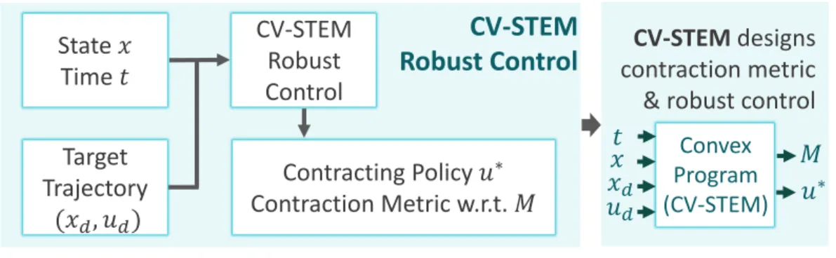
CV-STEM Control
As a result of Theorems 2.4, 2.5 and 3.1, the control law = 𝑢 an objective function for the CV-STEM control frame in the theorem. The convex minimization optimization problem (4.1), subject to the shrinkage constraint of Theorem 3.1, is given in Theorem 4.2, thus introducing CV-STEM control [1]–[4] for designing an optimal shrinkage metric and control policy of contracting as shown in Fig. The CV-STEM control weights 𝑐0 and 𝑐1 of Theorem 4.2 create a trade-off analogous to the LQR case with the cost weight matrices of 𝑄for the state and 𝑅 for the control, since the upper bound of the stable State tracking error (4.1) is proportional with 𝜒, and an upper bound of ∥𝐾∥ for the control gain 𝐾 in (3.10),𝑢=𝑢
CV-STEM Estimation
Note again that we can also use the SDC formulation with respect to a fixed point as delimited in Theorem 3.2 and as demonstrated in. The estimator (4.7) gives a convex steady-state upper bound on the Euclidean distance between 𝑥 and ˆ𝑥 as in Theorem. So by definition of 𝑐1 in Theorem 4.4, the greater the weight of 𝜈, the less confidence we have in 𝑦(𝑡) (see Example 4.2).
Control Contraction Metrics (CCMs)
Furthermore, Theorem 2.4 for deterministic perturbation rejection still holds and the CCM controller (4.22) possesses the same sense of optimality as for the CV-STEM controller in Theorem 4.2. We can consider the stochastic disturbance in Theorem 4.6 using Theorem 2.5, even with the differential control law of the form (4.22) or (4.24) as shown in [17]. Also, although relation (4.20) or (4.25) is not included as a constraint in Theorem 4.2 for simplicity of discussion, the dependence of 𝑊¤¯ on 𝑢 in Theorem 4.2 can be removed using it in a similar way to [17].
Remarks in CV-STEM Implementation
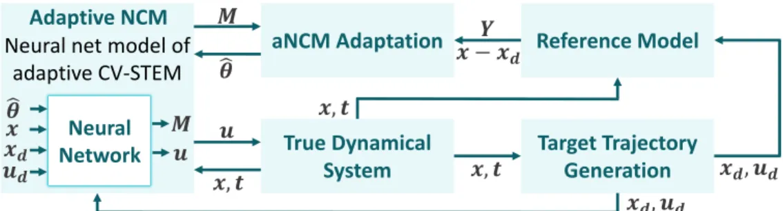
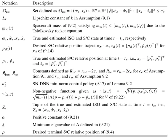
Note that these methods can be used in addition to the robust control approaches in the previous chapters. Assume that Assumption 8.1 holds and let M define the NCM of Definition 6.2, which models the CV-STEM contraction metric in Theorem 4.2 for the nominal system (8.1) with 𝜃 = 𝜃𝑛, constructed with an additional convex constraint. Let us recall the definitions of the ISO state flow and spacecraft state processes from Definitions 9.1 and 9.2 summarized in Table 9.2.
Contraction Theory for Learning-based Control
Problem Formulation
Consider the problem of learning a computationally expensive (or unknown) feedback control law 𝑢∗(𝑥 , 𝑥𝑑, 𝑢𝑑, 𝑡) that follows a target trajectory (𝑥𝑑, 𝑢𝑑) given by 𝑥¤𝑑 = 𝑓(𝑥𝑑, 𝑡) + 𝐵( 𝑥𝑑, 𝑡)𝑢𝑑 as in (3.3), assuming that 𝑓 and 𝐵 are known. Next, we consider the problem of learning a computationally expensive (or unknown) state estimator, approximating its score gain 𝐿(𝑥 , 𝑡ˆ ) by 𝐿𝐿(𝑥 , 𝑡ˆ ). Thus, condition (5.3) has become a common assumption in learning-based and data-driven performance analysis control technician.
Formal Stability Guarantees via Contraction Theory
The positive finality of 𝑀 could be exploited to reduce the dimension of the target DNN output due to the following lemma [1]. Since Lemma 8.1 guarantees the boundedness of ∥𝜃ˆ∥, the adaptive controller(8.8), 𝑢 =−K ( ¤q− ¤q𝑟) +𝑌 𝜃+𝑌𝜃˜, can be viewed as the exponentially stabilizing controller. This indeed indicates that the tracking error of the Lagrangian system (8.32) is exponentially bounded, as proven in Theorem 8.4.
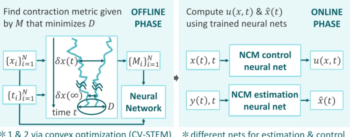
Learning-based Safe and Robust Control and Estimation
Stability of NCM-based Control and Estimation
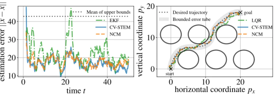
Assume that the systems (6.1) and (6.2) are controlled by𝑢𝐿, which computes the CV-STEM controller𝑢∗for Theorem 4.2 replacing𝑀 by M, i.e. Note that using the differential feedback control of Theorem 4.6 as 𝑢∗ also gives the bounds by the same argument [8]. It can be seen that the steady-state estimation errors of NCM and CV-STEM are below the optimal steady-state upper bound of Theorem 4.5 (dashed line on the left side of Fig. 6.2), while EKF has a larger error compared to the two others.
NCMs as Lyapunov Functions
6.2, NCM maintains its trajectories within the bounded error tube of Theorem 4.2 (shaded area) around the target trajectory (dashed line), avoiding collisions with circular obstacles, even in the presence of disturbances, while requiring much less computational cost than CV - STEM . As discussed in Remark 4.2, Theorem 6.5 can also be formulated in the stochastic setting as in Theorem 6.4 using the technique discussed in [8]. A similar estimation scheme based on the Ljapun function could be designed to estimate the state of CV-STEM and NCM in Theorems 4.5, 6.2 and 6.3, if its contraction constraints from Theorem 4.5 do not explicitly depend on the actual state 𝑥.
Remarks in NCM Implementation
We exploit the result of Theorem 7.1 in pipe-based motion planning [9] to generate LAG-ROS training data that satisfies the given state constraints even in the presence of learning error and disturbances from Theorem 5.2. 9.3, we train the SN-DNN to also minimize the deviation of the state trajectory with the SN-DNN guidance policy from the desired MPC state trajectory [4], [5]. This result can be considered as an extension of the minimum norm control methodology [29].
Learning-based Safe and Robust Motion Planning
Overview of Existing Motion Planners
In essence, our approach proposed in Theorem 7.1 to provide (a) stability guarantees based on the contraction theory (b), thereby significantly improving the performance of (a), which ensures only the tracking error ∥𝑥− 𝑥𝑑∥ to be bounded by a function that increases exponentially with time, as previously derived in Theorem 5.1 of Chapter 5.
Stability Guarantees of LAG-ROS
Due to its internal feedback structure, LAG-ROS achieves the exponential boundedness of trajectory tracking error as in Theorem 7.1, thereby improving the performance of existing learning-based feedforward control laws for modeling (𝑜ℓ, 𝑡) ↦→𝑢𝑑 as in (a), whose tracking error bound increases exponentially with time as in Theorem 5.1 (see [1]). LAG-ROS(c) and the robust pipeline planner (b) actually satisfy bound (7.4) (dotted black curve) for all 𝑡 with a small standard deviation 𝜎, unlike the learning-based motion planner (a) with divergent bound by Theorem 5.1 and increasing deflection 𝜎. As implied in Example 7.1, LAG-ROS indeed has guarantees for the robustness and stability of 𝑢∗ , as proved in Theorem 7.1, unlike (a), while maintaining a significantly lower computational cost than (b).
![Figure 7.2: Cart-pole balancing: 𝑥 = [ 𝑝, 𝜃 , 𝑝, ¤ 𝜃 ¤ ] ⊤ , 𝑥 and 𝑥 𝑑 are given in (6.1) and (6.3), (a) – (c) are given in Table 7.1, and 𝑟 ℓ is given in (7.4)](https://thumb-ap.123doks.com/thumbv2/123dok/10882766.0/131.918.203.718.113.315/figure-cart-pole-balancing-given-given-table-given.webp)
Tube-based State Constraint Satisfaction
The localization method in [2] allows extracting 𝑜ℓ from (a) with 𝑜𝑔 from (7.5), making LAG-ROS applicable to different environments in a distributed manner with a single policy. The robust control inputs for training LAG-ROS from Theorem 7.1 are then sampled by computing the CV-STEM from Theorem 4.2 or Theorem 4.6. LAG-ROS (c) addresses these two problems by providing formal robustness and stability guarantees of Theorem 7.1, while implicitly knowing the global solution (based only on the local information 𝑜ℓ as in [2]) without computing it online .
Safe Exploration and Learning of Disturbances
Collision Avoidance and Robust Tracking Augmentation
Improving the robustness performance here will simply lead to closer tracking of the safe trajectory 𝑥𝑑 (see the right side of Fig. 7.8) without losing too much information from the learned motion planning policy 𝑢𝑖. This framework therefore offers one way to ensure safety and robustness as in the LAG-ROS framework with Lemma 7.1 (see also [43]–[45] and references therein), which depends on the knowledge and the size of the approximation error of a given learned motion planning policy. The additional trace-based robust filter is for reducing the load of the safety filter in dealing with disturbances.
Theoretical Overview of CART
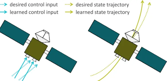
This provides an optimal and robust control input that minimizes its current deviation from the SN-DNN control policy, under the condition of gradual stability as in contraction theory [7]. It uses the known dynamics (9.1) and (9.2) to approximate an optimization-based guidance policy, thereby directly minimizing the deviation of the learned state trajectory from the optimal state trajectory with the smallest spacecraft delivery error at ISO rendezvous, which has a verifiable optimality gap with respect to to the optimal routing policy. As follows from Theorem 9.1, the SN-DNN minimum norm control policy (9.17) from Lemma 9.2 improves the SN-DNN terminal control policy from Lemma 9.1 by providing an explicit spacecraft delivery error bound (9.27) that is valid even under the presence of state uncertainty.
Learning-based Adaptive Control and Contraction Theory for
Learning-based Adaptive Control
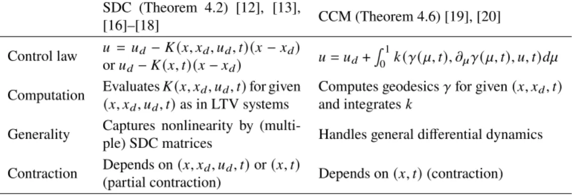
Note also that the techniques in this chapter [3] can be used with differential state feedback frameworks [4]-[9] as described in Theorem 4.6, which trades off extra computational cost for generality (see Tables 3.1 and . Although Theorem 8.1 applies the NCM designed to the nominal system (8.1) with 𝜃 = 𝜃𝑛, we could improve its representational power by explicitly taking the parameter estimate ˆ𝜃 as one of the NCM arguments [3], leading to the concept of an adaptive NCM (anNCM). Let us emphasize again that using Theorem 4.6, the results of Theorems 8.1 and 8.2 can be extended to adaptive control with CCM-based differential feedback, see Table 3.1 for trade-offs).
Contraction Theory for Learned Models
In particular, if we select 𝑥 as 𝑥 =[𝑝⊤,𝑝¤⊤]⊤ as its state, where 𝑝 ∈R3 is the position of the spacecraft relative to the ISO, we have that. Let us emphasize again that, as proven in Lemma 9.2, the deviation term𝑘(𝑥 ,ˆ œˆ, 𝑡) of the controller (9.17) is nonzero only if the stability condition (9.21) cannot be satisfied with the SN-DNN terminal . guidance policy 𝑢ℓ of Lemma 9.1. Before we move on to the next section on proving the robustness and stability properties of the SN-DNN min-norm check of (9.17) of Lemma 9.2, we need to make a few assumptions with the notations from Table 9.3, the first of which is that the spacecraft has access to an onboard navigation system that meets the following conditions.
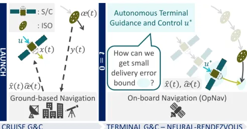
Interstellar Object Exploration
Technical Challenges in ISO Exploration
Note that the size of the neural network used is chosen to be small enough to significantly reduce the online computing load required to solve the optimization. The main design challenge here is how to give the learning approach a formal guarantee of meeting the ISO, ie. achieving a sufficiently small spacecraft delivery error given a given desired relative position for a flyby or ISO impact, leading to a problem formulated as follows. Our goal is to design an autonomous nonlinear G&C algorithm that robustly tracks the desired trajectory with zero spacecraft delivery error calculated using the above learning-based instructions and that provides bounded tracking error even in the presence of state uncertainty and learning error.
Autonomous Guidance via Dynamical System-Based Deep Learning 158
We will see how the choice of weights𝐶𝑢 and𝐶𝑥 affects the performance𝑢ℓ in Sect. Since the SN-DNN is Lipschitz bounded by design and robust to disturbances, the optimality gap of the guidance framework 𝑢ℓ introduced in Sect. S/C relative dynamics solution trajectory at time 𝑡 controlled by 𝑢ℓ without state estimation error, which satisfies𝜑𝜏.
Neural-Rendezvous: Learning-based Robust Guidance and Control
The bound 9.27 of Theorem 9.1 can be used as a tool to determine whether we should use the SN-DNN terminal guidance policy of Lemma 9.1 or the SN-DNN min norm checking policy (9.17) of Lemma 9.2, based on the trading in between, as you can see in the following. Terminal G&C (Neural-Rendezvous) is performed using the SN-DNN guidelines and the min-norm control policy online as in Algorithm 1, enabling fast-response autonomous operations under the high ISO status uncertainty and high-speed challenges. The SN-DNN terminal guidance policy of Lemma 9.1 can be implemented in real time and possesses an optimality gap as in (9.11), resulting in the near-.
Extensions
Additional Numerical Simulations and Empirical Validation
Numerical Simulations for ISO Exploration
Empirical Validation for ISO Exploration
Numerical Simulations for CASTOR
Concluding Remarks
Summary of Presented Methods
Future Plans