Costs - IPIEF FEB UMY

(1)

Chapter 6 Costs

(2)

2

Basic Concepts of Costs

 Opportunity cost is the cost of a good or service as measured by the alternative uses that are foregone by producing the good or service.

– If 15 bicycles could be produced with the materials used to produce an automobile, the opportunity cost of the automobile is 15 bicycles.

 The price of a good or service often may reflect its opportunity cost.

(3)

3

Basic Concepts of Costs

 Accounting cost is the concept that goods or services cost what was paid for them.

 Economic cost is the amount required to keep a resource in its present use; the amount that it would be worth in its next best alternative use.

(4)

4

Labor Costs

 Like accountants, economists regard the payments to labor as an explicit cost.

 Labor services (worker-hours) are purchased at an hourly wage rate (w): The cost of hiring one worker for one hour.

 The wage rate is assumed to be the amount workers would receive in their next best

alternative employment.

(5)

5

Capital Costs

 While accountants usually calculate capital

costs by applying some depreciation rule to the historical price of the machine, economists

view this amount as a sunk cost.

 A sunk cost is an expenditure that once made cannot be recovered.

 These costs do not focus on foregone opportunities.

(6)

6

Capital Costs

 Economists consider the cost of a machine to be the amount someone else would be willing to pay for its use.

 The cost of capital services (machine-hours) is the rental rate (v) which is the cost of hiring one machine for one hour.

 This is an implicit cost if the machine is owned by the firm.

(7)

7

Two Simplifying Assumptions

 The firm uses only two inputs: labor (L, measured in labor hours) and capital (K, measured in machine hours).

– Entrepreneurial services are assumed to be included in the capital costs.

 Firms buy inputs in perfectly competitive markets so the firm faces horizontal supply curves at prevailing factor prices.

(8)

8

Economic Profits and Cost Minimization

 Total costs = TC = wL + vK.

 Assuming the firm produces only one output, total revenue equals the price of the product

(P) times its total output [q = f(K,L) where f(K,L) is the firm’s production function].

(9)

9

Economic Profits and Cost Minimization

 Economic profits () is the difference

between a firm’s total revenues and its total economic costs.

. )

, (

costs Total

- revenues Total

vK wL

L K

Pf

vK wL

Pq









 

(10)

10

Cost-Minimizing Input Choice

 Assume, for purposes of this chapter, that the firm has decided to produce a particular output level (say, q₁).

– The firm’s total revenues are P·q₁.

 How the firm might choose to produce this

level of output at minimal costs is the subject of this chapter.

(11)

11

Cost-Minimizing Input Choice

 Cost minimization requires that the marginal rate of technical substitution (RTS) of L for K equals the ratio of the inputs’ costs, w/v:

v

RTS ( of L for K)  w

(12)

12

Graphic Presentation

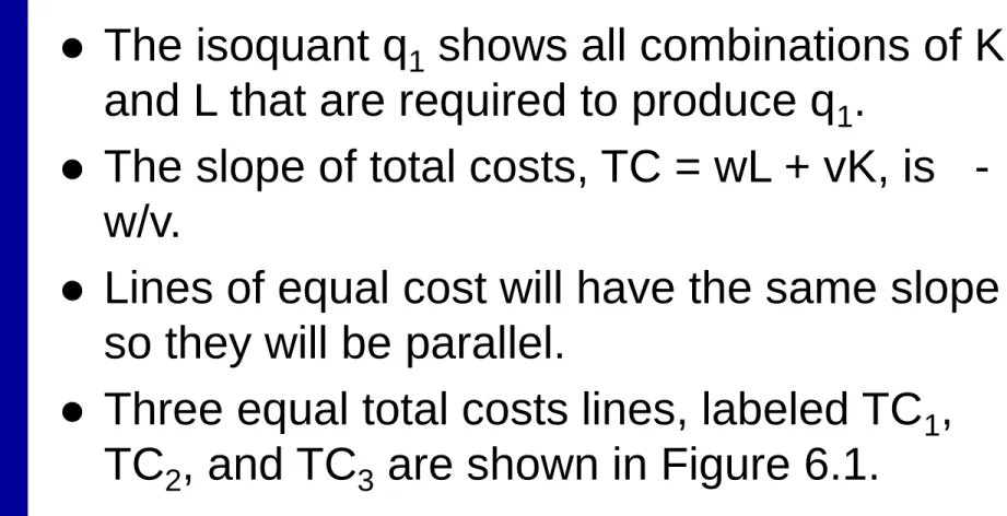
 The isoquant q₁ shows all combinations of K and L that are required to produce q₁.

 The slope of total costs, TC = wL + vK, is - w/v.

 Lines of equal cost will have the same slope so they will be parallel.

 Three equal total costs lines, labeled TC₁, TC₂, and TC₃ are shown in Figure 6.1.

(13)

Capital per week

TC₁

TC₂

TC₃

q₁ K*

Labor per week 0 L*

(14)

14

Graphic Presentation

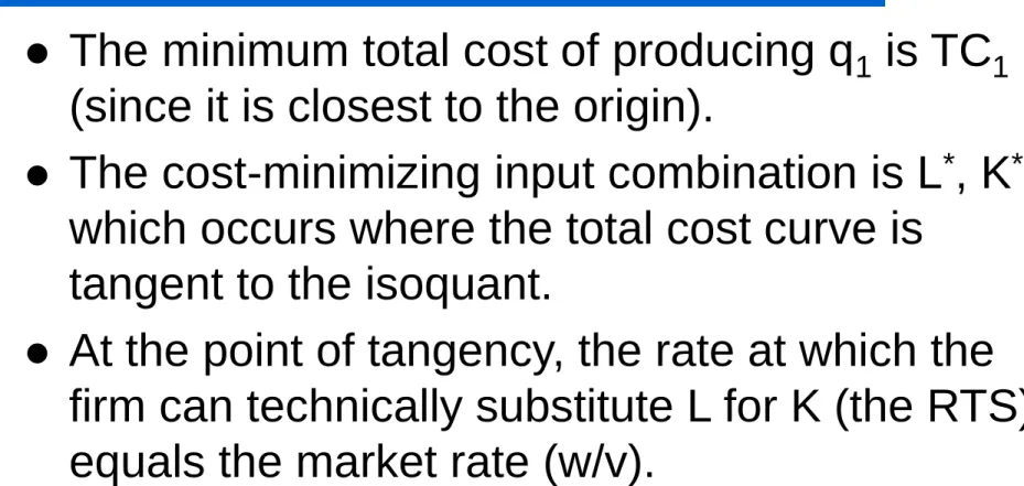
 The minimum total cost of producing q₁ is TC₁ (since it is closest to the origin).

 The cost-minimizing input combination is L^*, K^* which occurs where the total cost curve is

tangent to the isoquant.

 At the point of tangency, the rate at which the firm can technically substitute L for K (the RTS) equals the market rate (w/v).

(15)

15

An Alternative Interpretation

. ,

. K)

for L

of (

v MP w

MP

v w MP

RTS MP

MP RTS MP

K L



 From Chapter 5 

 Cost minimization requires

 or, rearranging

(16)

16

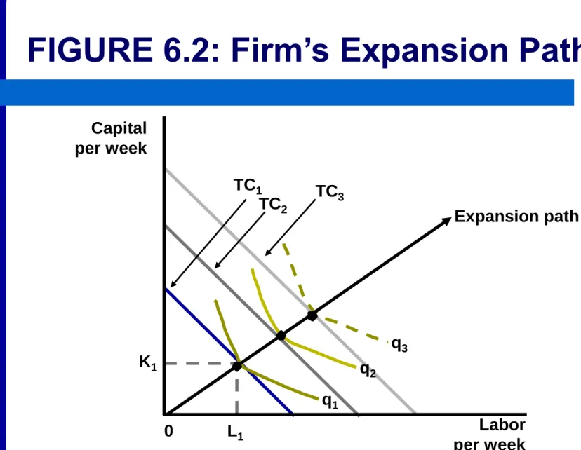
The Firm’s Expansion Path

 A similar analysis could be performed for any output level (q).

 If input costs (w and v) remain constant, various cost-minimizing choices can be traces out as shown in Figure 6.2.

 For example, output level q₁ is produced

using K₁, L₁, and other cost-minimizing points are shown by the tangency between the total cost lines and the isoquants.

(17)

17

The Firm’s Expansion Path

 The firm’s expansion path is the set of cost- minimizing input combinations a firm will

choose to produce various levels of output (when the prices of inputs are held constant).

 Although in Figure 6.2, the expansion path is a straight line, that is not necessarily the case.

(18)

18

TC₁ TC₃ TC₂

Expansion path

q₁

q₂ q₃ K₁

Labor per week L₁

0

FIGURE 6.2: Firm’s Expansion Path

(19)

19

Cost Curves

 A firm’s expansion path shows how minimum- cost input use increases when the level of

output expands.

 With this it is possible to develop the

relationship between output levels and total input costs.

 These cost curves are fundamental to the theory of supply.

(20)

20

Cost Curves

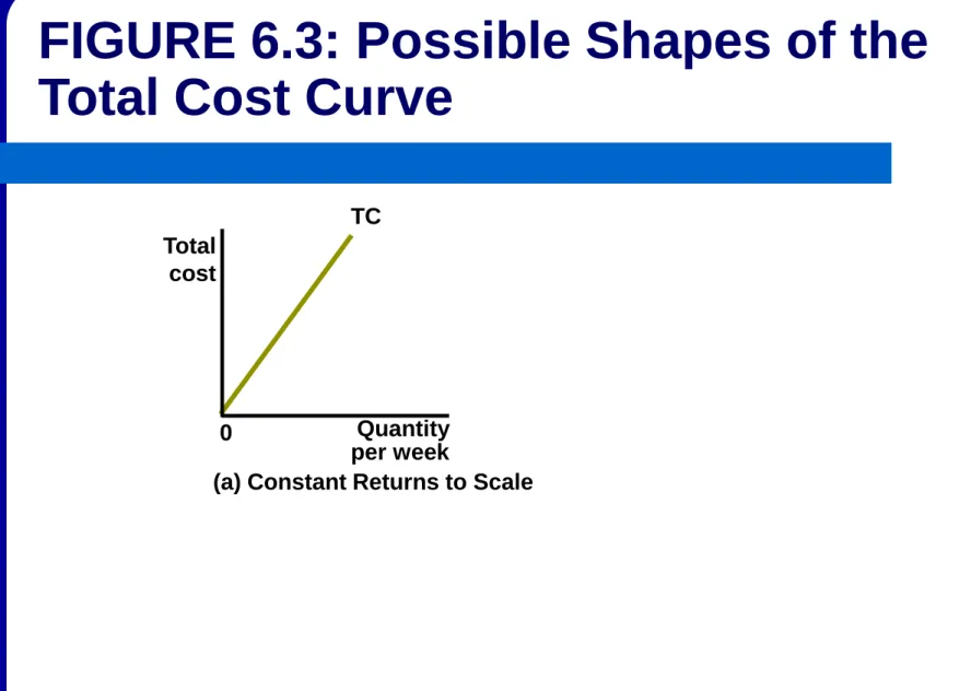
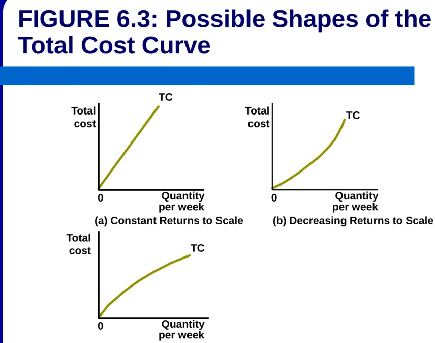
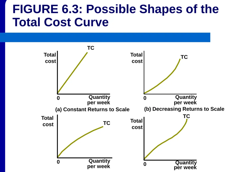
 Figure 6.3 shows four possible shapes for cost curves.

 In Panel a, output and required input use is proportional which means doubling of output requires doubling of inputs. This is the case when the production function exhibits constant returns to scale.

(21)

21

Total cost

TC

Quantity per week

(a) Constant Returns to Scale 0

FIGURE 6.3: Possible Shapes of the

Total Cost Curve

(22)

22

Cost Curves

 Panels b and c reflect the cases of decreasing and increasing returns to scale, respectively.

 With decreasing returns to scale the cost curve is convex, while the it is concave with

increasing returns to scale.

 Decreasing returns to scale indicate

considerable cost advantages from large scale operations.

(23)

23

Total cost

TC

Total

cost TC

(b) Decreasing Returns to Scale 0

Total

cost TC

(c) Increasing Returns to Scale 0

FIGURE 6.3: Possible Shapes of the

Total Cost Curve

(24)

24

Cost Curves

 Panel d reflects the case where there are increasing returns to scale followed by

decreasing returns to scale.

 This might arise because internal co-ordination and control by managers is initially

underutilized, but becomes more difficult at high levels of output.

 This suggests an optimal scale of output.

(25)

25

Total cost

TC

Total

cost TC

Total

cost TC

Total cost

TC

Quantity per week (d) Optimal Scale 0

FIGURE 6.3: Possible Shapes of the

Total Cost Curve

(26)

26

Average Costs

 Average cost is total cost divided by output; a common measure of cost per unit.

 If the total cost of producing 25 units is $100, the average cost would be

q AC  TC

 cost Average

4 25 $

100

$ 

 AC

(27)

27

Marginal Cost

 The additional cost of producing one more unit of output is marginal cost.

 If the cost of producing 24 units is $98 and the cost of producing 25 units is $100, the marginal cost of the 25^th unit is $2.

q in Change

TC in

Change cost

Marginal  MC 

(28)

28

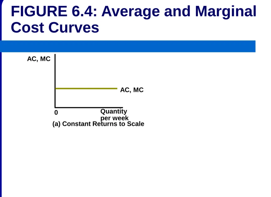
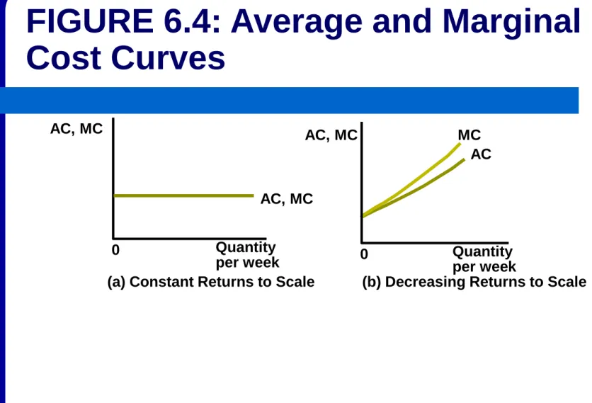
Marginal Cost Curves

 Marginal costs are reflected by the slope of the total cost curve.

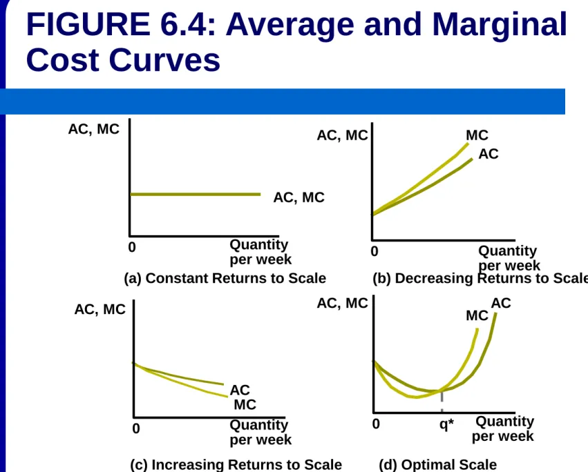
 The constant returns to scale total cost curve shown in Panel a of Figure 6.3 has a constant slope, so the marginal cost is constant as

shown by the horizontal marginal cost curve in Panel a of Figure 6.4.

(29)

29

AC, MC

Quantity per week (a) Constant Returns to Scale

0

FIGURE 6.4: Average and Marginal

Cost Curves

(30)

30

Marginal Cost Curves

 With decreasing returns to scale, the total cost curve is convex (Panel b of Figure 6.3).

 This means that marginal costs are increasing which is shown by the positively sloped

marginal cost curve in Panel b of Figure 6.4.

(31)

31

AC, MC

0

AC, MC

AC MC

FIGURE 6.4: Average and Marginal

Cost Curves

(32)

32

Marginal Cost Curves

 Increasing returns to scale results in a concave total cost curve (Panel c of Figure 6.3).

 This causes the marginal costs to decrease as output increases as shown in the negatively

sloped marginal cost curve in Panel c of Figure 6.4.

(33)

33

AC, MC

0

AC, MC

AC

MC

AC, MC

FIGURE 6.4: Average and Marginal

Cost Curves

(34)

34

Marginal Cost Curves

 When the total cost curve is first concave followed by convex as shown in Panel d of

Figure 6.3, marginal costs initially decrease but eventually increase.

 Thus, the marginal cost curve is first negatively sloped followed by a positively sloped curve as shown in Panel d of Figure 6.4.

(35)

35

AC, MC

0

AC, MC

AC

MC

AC, MC

Quantity per week (d) Optimal Scale

0 q*

FIGURE 6.4: Average and Marginal

Cost Curves

(36)

36

Average Cost Curves

 If a firm produces only one unit of output,

marginal cost would be the same as average cost

 Thus, the graph of the average cost curve begins at the point where the marginal cost curve intersects the vertical axis.

(37)

37

Average Cost Curves

 For the constant returns to scale case,

marginal cost never varies from its initial level, so average cost must stay the same as well.

 Thus, the average cost curve are the same horizontal line as shown in Panel a of Figure 6.4.

(38)

38

Average Cost Curves

 With convex total costs and increasing

marginal costs, average costs also rise as shown in Panel b of Figure 6.4.

 Because the first few units are produced at low marginal costs, average costs will always b

less than marginal cost, so the average cost curve lies below the marginal cost curve.

(39)

39

Average Cost Curves

 With concave total cost and decreasing marginal costs, average costs will also

decrease as shown in Panel c in Figure 6.4.

 Because the first few units are produced at relatively high marginal costs, average is less than marginal cost, so the average cost curve lies below the marginal cost curve.

(40)

40

Average Cost Curves

 The U-shaped marginal cost curve shown in Panel d of Figure 6.4 reflects decreasing

marginal costs at low levels of output and increasing marginal costs at high levels of output.

 As long as marginal cost is below average cost, the marginal will pull down the average.

(41)

41

Average Cost Curves

 When marginal costs are above average cost, the marginal pulls up the average.

 Thus, the average cost curve must intersect the marginal cost curve at the minimum

average cost; q^* in Panel d of Figure 6.4.

 Since q^* represents the lowest average cost, it represents an “optimal scale” of production for the firm.

(42)

42

Distinction between the Short Run and the Long Run

 The short run is the period of time in which a firm must consider some inputs to be

absolutely fixed in making its decisions.

 The long run is the period of time in which a firm may consider all of its inputs to be variable in making its decisions.

(43)

43

Holding Capital Input Constant

 For the following, the capital input is assumed to be held constant at a level of K₁, so that,

with only two inputs, labor is the only input the firm can vary.

 As examined in Chapter 5, this implies diminishing marginal productivity to labor.

(44)

44

Types of Short-Run Costs



Fixed costs; costs associated with inputs that are fixed in the short run.



Variable costs; costs associated with

inputs that can be varied in the short

run.

(45)

45

Input Inflexibility and Cost Minimization

 Since capital is fixed, short-run costs are not the minimal costs of producing variable output levels.

 Assume the firm has fixed capital of K₁ as shown in Figure 6.5.

 To produce q₀ of output, the firm must use L₁ units of labor, with similar situations for q₁, L₁, and q₂, L₂.

(46)

46

STC₀ STC₁ STC₂

q₁

q₂

q₀ K₁

Labor per week

L₀ L₁ L₂

0

FIGURE 6.5: “Nonoptimal” Input

Choices Must Be Made in the Short Run

(47)

47

Input Inflexibility and Cost Minimization

 The cost of output produced is minimized

where the RTS equals the ratio of prices, which only occurs at q₁, L₁.

 Q₀ could be produce at less cost if less capital than K₁ and more labor than L₀ were used.

 Q₂ could be produced at less cost if more capital than K₁ and less labor than L₂ were used.

(48)

48

Per-Unit Short-Run Cost Curves

q in Change

STC in

Change cost

marginal run

- Short and

cost average

run -

Short



SMC

q

SAC STC

(49)

49

Per-Unit Short-Run Cost Curves

 Having capital fixed in the short run yields a total cost curve that has both concave and convex sections, the resulting short-run

average and marginal cost relationships will also be U-shaped.

 When SMC < SAC, average cost is falling, but when SMC > SAC average cost increase.

(50)

50

Relationship between Short-Run and Long-Run per-Unit Cost Curves

 Figure 6.6 shows all cost relationships for a firm that has U-shaped long-run average and marginal cost curves.

 At output level q^* long-run average costs are minimized and MC = AC.

 Associated with q^* is a certain level of capital, K^*.

(51)

51

SMC MC

SAC

AC AC, MC

0 q*

FIGURE 6.6: Short-Run and Long-Run Average and Marginal Cost Curves at Optimal Output Level

(52)

52

Relationship between Short-Run and Long-Run per-Unit Cost Curves

 In the short-run, when the firm using K^* units of capital produces q^*, short-run and long-run

total costs are equal.

 In addition, as shown in Figure 6.6 AC = MC = SAC(K^*) = SMC(K^*).

 For output above q^* short-run costs are higher than long-run costs. The higher per-unit costs reflect the facts that K is fixed.

(53)

53

Shifts in Cost Curves

 Any change in economic conditions that affects the expansion path will also affect the shape

and position of the firm’s cost curves.

 Three sources of such change are:

– change in input prices

– technological innovations, and

– economies of scope.

(54)

54

Changes in Input Prices

 A change in the price of an input will tilt the firm’s total cost lines and alter its expansion path.

 For example, a rise in wage rates will cause

firms to use more capital (to the extent allowed by the technology) and the entire expansion

path will rotate toward the capital axis.

(55)

55

Changes in Input Prices

 Generally, all cost curves will shift upward with the extent of the shift depending upon how

important labor is in production and how successful the firm is in substituting other inputs for labor.

– With important labor and poor substitution

possibilities, a significant increase in costs will result.

(56)

56

Technological Innovation

 Because technological advances alter a firm’s production function, isoquant maps as well as the firm’s expansion path will shift when

technology changes.

 Unbiased improvements would shift isoquants toward the origin enabeling firms to produce the same level of output with less of all inputs.

(57)

57

Technological Innovation

 Technological change that is biased toward the use of one input will alter isoquant maps, shift expansion paths, and affect the shape and

location of cost curves.

– For example, if workers became more skilled, this would save only on labor input.

(58)

58

Economies of Scope

 Economies of scope is the reduction in the costs of one product of a multiproduct firm when the output of another product is

increased.

– For example, when hospitals do many surgeries of one type, it may have cost advantages in doing

other types because of the similarities in equipment and operating personnel used.

(59)

59

A Numerical Example

 Assume Hamburger Heaven (HH) can hire workers at $5 per hour and it rents all of its grills for $5 per hour.

 Total costs for HH during one hour are TC = 5K + 5L

where K and L are the number of grills and the number of workers hired during that hour,

respectively.

(60)

60

A Numerical Example

 Suppose HH wishes to produce 40 hamburgers per hour.

 Table 6.1 repeats the various ways HH can produce 40 hamburgers per hour.

– This shows that total costs are minimized when K = L = 4.

 Figure 6.10 shows the cost-minimizing tangency.

(61)

61

TABLE 6.1: Total Costs of Producing 40 Hamburgers per Hour

Output (q) Workers (L) Grills (K) Total Cost (TC)

40 1 16.0 $85.00

40 2 8.0 50.00

40 3 5.3 41.50

40 4 4.0 40.00

40 5 3.2 41.00

40 6 2.7 43.50

40 7 2.3 46.50

40 8 2.0 50.00

40 9 1.8 54.00

40 10 1.6 58.00

(62)

62

Grills per hour

2 8

4

Workers per hour

40 hamburgers per hour E

Total cost = $40

2 4 8

0

Figure 6.7: Cost-Minimizing Input

Choice for 40 Hamburgers per Hour

(63)

63

Long-Run cost Curves

 HH’s production function is constant returns to scale so

 As long as w = v = $5, all of the cost

minimizing tangencies will resemble the one shown in Figure 6.10 and long-run cost

minimization will require K = L.

(64)

64

Long-Run cost Curves

 This situation, resulting from constant returns to scale, is shown in Figure 6.8.

 HH’s long-run total cost function is a straight line through the origin as shown in Panel a.

 Its long-run average and marginal costs are constant at $1 per burger as shown in Panel b.

(65)

65

Total costs

20 60

$80

40

Total costs

40 60

20 80

(a) Total Costs

0

Average and marginal costs

$1.00

Hamburgers per hour 40 60

20 80

(b) Average and Marginal Costs

0

FIGURE 6.8: Total, Average, and Marginal Cost Curves

Average and marginal costs Hamburgers

per hour

(66)

66

Short-Run Costs

 Table 6.2 repeats the labor input required to produce various output levels holding grills fixed at 4.

 Diminishing marginal productivity of labor

causes costs to rise rapidly as output expands.

 Figure 6.9 shows the short-run average and marginal costs curves.

(67)

67

TABLE 6.2: Short-Run Costs of Hamburger Production

Output (q)

Workers (L)

Grills (K)

Total Cost (STC)

Average Cost (SAC)

Marginal Cost (SMC)

10 0.25 4 $21.25 $2.125 -

20 1.00 4 25.00 1.250 $0.50

30 2.25 4 31.25 1.040 0.75

40 4.00 4 40.00 1.000 1.00

50 6.25 4 51.25 1.025 1.25

60 9.00 4 65.00 1.085 1.50

70 12.25 4 81.25 1.160 1.75

80 16.00 4 100.00 1.250 2.00

90 20.25 4 121.25 1.345 2.25

100 25.00 4 145.00 1.450 2.50

(68)

68

Average and marginal costs

.50 1.00

$2.50

2.00 1.50

Hamburgers per hour SMC (4 grills)

SAC (4 grills)

AC, MC

40

20 60 80 100

0

FIGURE 6.12: Short-Run and Long-Run Average and Marginal Cost Curves for Hamburger Heaven