John is also visiting professor at the University of the West of England, Bristol, where he was Head of the School of Economics from 1992 to 1999. In 2006, Dean received an Outstanding Teaching Award from the Economics Network of the Higher Education Academy.
Part F MACROECONOMIC MODELS, THEORIES AND POLICY
Supporting Resources
Custom Publishing
Preface
A NOTE TO THE STUDENT FROM THE AUTHORS
TO LECTURERS AND TUTORS
Extensive revision
SUGGESTIONS FOR SHORTER OR LESS ADVANCED COURSES
Less advanced but comprehensive courses
Economics for Business courses
Introduction to microeconomics
Introduction to macroeconomics
Outline courses
Courses with a theory bias
Courses with a policy bias (and only basic theory)
COMPANION RESOURCES
MyEconLab (for students)
MyEconLab (for lecturers)
Additional resources for lecturers
Acknowledgements
Publisher’s Acknowledgements
Text
Part
Introduction
Why Economics is Good for You
WHAT IS ECONOMICS?
An island economy
Books and media
A pay-rise, how exciting
Of course I want to know
We need to save more; we need to spend more
PUZZLES AND STORIES
APPLYING THE PRINCIPLES
Thinking like an economist – a word of warning
Economics and Economies
WHAT DO ECONOMISTS STUDY? 7
WHAT DO ECONOMISTS STUDY?
The problem of scarcity
Definitions
Of course, not all of us face the problem of scarcity to the same extent. In fact, this is one of the main issues that economists study: how resources are distributed, whether among different individuals, different regions of a country or different countries of the world.
Demand and supply
A poor family who may not be able to eat enough or afford a decent place to stay will hardly see it as a 'problem' that a rich family cannot afford a second skiing holiday. This economic problem – limited resources but unlimited needs – makes people, rich and poor alike, behave in certain ways.
Dividing up the subject
WHAT DO ECONOMISTS STUDY? 9 spending in the economy, whether by consumers, by cus-
It deals with the supply and demand of certain goods, services and resources, such as cars, butter, clothing, haircuts, plumbers, accountants, blast furnaces, computers and oil. Which of the following issues are macroeconomic issues, which are microeconomic issues, and which may depend on the context?
Macroeconomics
Microeconomics Microeconomics and choice
Assessing different countries’ macroeconomic performance
WHAT DO ECONOMISTS STUDY? 11 more food a nation produces, the fewer resources will there
In other words, the production or consumption of one thing involves the sacrifice of alternatives. This sacrifice of alternatives in the production (or consumption) of a good is known as its opportunity cost.
WHAT DO ECONOMISTS STUDY? 13
In any economic activity, allocative efficiency will increase as long as more of that activity (and therefore fewer alternatives) involve greater marginal benefit than marginal cost. Throughout the book, we will think about how a good economy fulfills various economic and social goals, micro or macro.
Illustrating economic issues: the production possibility curve
Opportunity cost is the sacrifice made by going to university or college instead of doing something else. Is the opportunity cost to the individual of pursuing higher education different from the opportunity cost to society as a whole.
Buying a textbook costing £59.99
If there are several other things you could have done, the opportunity costs the sum of all these things. You may not have realized it, but you probably think about opportunity costs many times a day.
Coming to lectures
What you should know to make an informed decision about what to do that evening. We are constantly making decisions: what to buy, what to eat, what to wear, whether to go out, how much to study, etc.
Choosing to study at university or college
WHAT DO ECONOMISTS STUDY? 15
The opportunity cost of five million units of clothing is 1 million units of food. The opportunity cost of six million units of clothing is 2 million units of food.
Water
WHAT DO ECONOMISTS STUDY? 17
This growth in potential output is illustrated by an outward shift in the production possibility curve.
Illustrating economic issues: the circular flow of goods and incomes
This flow diagram, like the production possibility curve, can help us distinguish between microeconomics and macroeconomics. Macroeconomics deals with the total size of the flow and what causes it to expand and contract.
Section summary
Thus, labor services and other factors flow from households to firms, and in exchange firms pay money to households – namely wages, rents, dividends and interest. Microeconomics deals with the composition of the circular flow: what combinations of goods make up the flow of goods; how the various factors of production combine to produce that good; for which wages, dividends, rents and interest are paid.
Firms demand the use of factors of production owned by households – labour, land and capital. Just as we referred to specific goods markets, so we can also refer to specific factor markets – the market for masons, for football players, for land, and so on.
The classification of economic systems
DIFFERENT ECONOMIC SYSTEMS 19
In practice, all economies are a mixture of the two; it is the degree of government intervention that distinguishes different economic systems. The diagram is useful in that it provides a simple picture of the mix of government and the market that exists in various economies.
Definition
The relative size of the informal sector varies from country to country and over time. What was once part of the informal sector is now part of the market sector.
The command economy
In many developing countries, much of the economic activity in poorer areas involves subsistence production. While some of the raw materials (eg building materials) may have to be purchased through the market, much of this production is in the informal sector and involves no exchange of money.
Assessment of the command economy
DIFFERENT ECONOMIC SYSTEMS 21
The workers would have no choice where to work; consumers would have no choice in what to buy. A shortage will occur if consumers decide to buy more; profits will arise if they decide to buy less.
The free-market economy Free decision making by individuals
Most of these problems were experienced in the former Soviet Union and other Eastern bloc countries and were part of the reason for the overthrow of their communist regimes (see Box 1.5. Initially, the disruption of market movement led to a decline in the Russian economy.
Russia
DIFFERENT ECONOMIC SYSTEMS 23
An increase in the supply of the good causes an increase in the demand for the factors of production (i.e. inputs) used in its production. The resulting surplus will lower the price of the good, which will encourage consumers to buy more.
China
This will lower the production costs of companies using these raw materials and increase the supply of finished products. Although all individuals in a free market economy look only to their own interests, the incentives of the price mechanism actually encourage them to respond to the wishes of others.
Assessment of the free-market economy
DIFFERENT ECONOMIC SYSTEMS 25
The mixed economy
THE NATURE OF ECONOMIC REASONING 27 The fact that government intervention can be used to rec-
However, a command economy is likely to be inefficient and bureaucratic; prices and the choice of production methods are likely to be arbitrary; incentives may be inappropriate; deficits and surpluses may arise. In practice, however, competition may be limited; there can be great inequality; there may be adverse social and environmental consequences; there may be macroeconomic instability.
The economic systems of different countries differ depending on the extent to which they rely on the market or the government to allocate resources. It is the degree and form of government intervention that distinguishes one type of economy from another.
Economics as a science
Due to the complexity of the real world, economic models must make several simplifying assumptions. Due to a lack of conclusive evidence about exactly how many parts of the economy are functioning, economists also need detective skills.
Economics as a social science
THE NATURE OF ECONOMIC REASONING 29 will fall by 10 per cent, only that total demand will. Some
As we will see later in the book, different political parties may adhere to different schools of economic thought. The fact that there are different economic theories does not mean that economists always disagree.
Economics and policy
How will people respond to a crisis, such as the global banking and credit crisis of 2007-8. For these reasons, competing models of economics abound, each making different assumptions and leading to different policy conclusions.
END OF CHAPTER QUESTIONS
Online resources
Additional case studies in MyEconLab
Websites relevant to this chapter
Foundations of Microeconomics
Supply and Demand
DEMAND 35 The markets we will be examining are highly competitive
In the case of consumers, this means accepting the prices that apply to the things they buy. One reason is that they provide a useful approximation to the real world and give us many insights into how a market economy works.
In the case of firms, perfect competition means that producers are small and face too much competition from other firms to be able to raise prices. They will still have to consider overall consumer demand and their competitors' prices.
The relationship between demand and price
In most cases this is true; when you get to the supermarket checkout, you can't start haggling with the cashier about the price of a can of beans or a tub of ice cream. They refer to the amount that consumers are willing and able to buy at a given price during a given period (eg week, month or year).
The demand curve
DEMAND 37
What explanations might there be for the very different shapes of their two demand curves? In textbooks, demand curves (and other curves as well) are only occasionally used to present specific data.
Other determinants of demand
If the price of bicycles falls, which leads to more purchases, the demand for inner tubes will increase. If national income were redistributed from the poor to the rich, the demand for luxury goods would increase.
Movements along and shifts in the demand curve
DEMAND 39
LOOKING AT THE MATHS
DEMAND 41 CASE STUDIES AND
Using equation (3) and the table below, calculate the following for 2010:. a) price elasticity of demand for lamb;. The relationship between quantity demanded and various determinants of demand (including price) can be expressed as an equation.
When the price of a good rises, the quantity demanded will fall over a period of time. The relationship between price and demand over time can be shown in a table (or "schedule") or as a graph.
Supply and price
On the graph, price is plotted on the vertical axis and quantity demanded per period on the horizontal axis. Other determinants of demand include taste, the number and price of substitute goods, the number.
The supply curve
SUPPLY 43
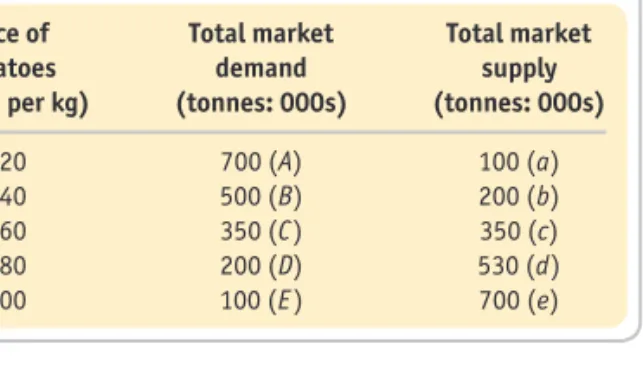
A supply curve can be the supply curve of an individual company, or a market curve (that is, that of the entire industry). For example, a price increase from 60 pence per kilogram to 80 pence per kilogram will cause a movement along the supply curve from point c to point d: the total market supply will rise from 350,000 tons per month to 530,000 tons per month.
Other determinants of supply
If more petrol is produced as a result of an increase in demand and therefore price, the supply of these other fuels will also increase. By referring to each of the above determinants of supply, you can determine what would cause (a) the supply of potatoes to decrease and (b) the supply of leather to increase.
Movements along and shifts in the supply curve
PRICE AND OUTPUT DETERMINATION 45
If a determinant other than price changes, the effect is shown by a shift in the entire supply curve. The relationship between the quantity supplied and the various determinants of supply can be expressed in the form of an equation.
There are two short-run reasons why a higher price encourages producers to supply more: (a) they are now willing to incur the higher cost per unit that comes with producing more; (b) they will switch to producing this product and away from products that are now less profitable. The relationship between price and quantity supplied per period can be shown in a table (or schedule) or as a graph.
Equilibrium price and output
PRICE AND OUTPUT DETERMINATION 47
Partial equilibrium
Movement to a new equilibrium
PRICE AND OUTPUT DETERMINATION 49
Problems in identifying the position and shape of the demand curve: shift in demand and supply curves Figure 2.9. Problems identifying the position and shape of the demand curve: only shift in the supply curve.
Incentives in markets
In Figure 2.9, however, not only has the supply curve shifted, but the demand curve has also shifted. Is the change in price and quantity entirely due to the shift in the demand curve, or has the supply curve also shifted.
Identifying the position of demand and supply curves
The problem is that when the supply curve shifts, we often have no way of knowing whether or not the demand curve has shifted and by how much. For example, it is difficult to identify the shape of the demand curve simply by observing price and quantity if it is not known whether changes in other determinants have shifted the demand curve.
The ups and downs (and ups again) of the housing market
The determinants of house prices
PRICE AND OUTPUT DETERMINATION 51 CASE STUDIES AND
Those who had houses for sale waited until the last possible moment, hoping to get a higher price. The net effect was a rightward shift of the housing demand curve and a leftward shift of the supply curve.
What of the future?
The effect of this speculation was to worsen the price change again - this time to a fall in prices. Speculation has increased in recent years due to the growth of the buy-to-let industry, with mortgage lenders entering the market in large numbers and a huge amount of media attention focused on individuals' potential for very high returns.
Demand
PRICE AND OUTPUT DETERMINATION 53 CASE STUDIES AND
The rise and fall in stock prices associated with expectations mirror those in the housing market and are discussed in Box 2.2. As the recession deepened and as more news came out about the banks. Bad debts built up, keeping stock prices volatile until a bullish trend started after the worst of the downturn had passed.
Supply
Then with the credit crunch and falling profits from 2007 share prices fell, with the falls resulting in further selling and further declines as confidence declined. However, with a bank bailout announced by governments around the world (see Box 18.3), expectations turned more positive, and the FTSE rose 17 percent in just two days.
Share prices and business
Things reached a crisis point in October 2008 when people feared the banks would fail and the recession would begin.
So it’s important to get them right
Financial and non-financial incentives
Do incentives lead to desirable outcomes?
THE CONTROL OF PRICES 55
The price cannot fall below this level (although it can rise above it). The price cannot rise above this level (although it is allowed to fall below it).
Setting a minimum (high) price
Setting a maximum (low) price
THE CONTROL OF PRICES 57
What would be the effect on underground market prices of an increase in the official price? Is there any truth to the saying that the price of a good is a reflection of its quality?
Markets in Action
ELASTICITY 61
Price elasticity of demand
Measuring the price elasticity of demand
Interpreting the figure for elasticity The use of proportionate or percentage measures
Determinants of price elasticity of demand
Over the next few months, there was only a very small reduction in the consumption of petroleum products. Indeed, within months there were signs that these effects were beginning to emerge as demand for large, fuel-heavy cars in the US (such as Hummers and other SUVs) fell and demand for smaller European and Japanese models increased.
Price elasticity of demand and consumer expenditure
Any increase in price will be exactly offset by a decrease in quantity, leaving the total consumer. The reason for its shape is that the proportional increase in quantity must equal the proportional decrease in price (and vice versa).
The measurement of elasticity: arc elasticity
You might think that a demand curve with unit elasticity would be a straight line angled at 45° to the axes. As we move along the demand curve, to keep the proportional change in both price and quantity constant, there must be an ever greater absolute increase in quantity and a smaller and smaller absolute fall in price.
Shifting the demand curve to the right
Making the demand curve less elastic
ELASTICITY 67 CASE STUDIES AND
Pricing on the buses
The measurement of elasticity
At any point on the demand curve, dP / dQ is given by the slope of the curve (the rate of its change). The slope is found by drawing a tangent to the curve at that point and finding the slope of the tangent.
Elasticity of a straight-line demand curve
ELASTICITY 69
BOX 3.3 USING CALCULUS TO CALCULATE THE PRICE ELASTICITY OF DEMAND ECONOMICS EXPLORING
ELASTICITY 71
Income elasticity of demand
ELASTICITY 73
Note that this is a 'linear' equation because it has no power terms, such as P 2 or Y 2. This is the convention when the equation contains more than one independent variable (in this case P A , Y and P B.
Similarly, the formula for the cross-price elasticity of demand for good A with respect to good B will be. Cross-price elasticity of demand measures the responsiveness of demand for one good to a change in the price of another.
Elasticity is a measure of the responsiveness of demand (or supply) to a change in one of the determinants. Since demand curves are downward sloping, the price elasticity of demand will have a negative value.
Short-run and long-run adjustment
Price expectations and speculation
THE TIME DIMENSION 77
This time, believing that the drop in price heralds further drops in price to come, suppliers sell now before the price drops. Redraw Figures 3.14 and 3.15 assuming, as in the previous question, that the initial change in price was caused by a shift in the supply curve.
Dealing with uncertainty and risk
This is most likely in times of uncertainty, when there are significant changes in the determinants of supply and demand. They 'jump on the bandwagon' and do what the rest are doing, further fueling the rise or fall in price.
Is short selling always profitable?
Concerns that the practice of short selling leads to instability in financial markets have led a number of governments – or agencies acting on their behalf – to ban the practice. In May 2010, the German government introduced a ban on short selling of all EU sovereign debt and bank stocks, and in August 2011 various European countries banned short selling of bank stocks following dramatic declines in bank share prices.
Short selling in the banking crisis of 2008
THE TIME DIMENSION 79
A way of reducing uncertainty
Speculators
Sellers
Buyers
The determination of the future price
At the time when they sow wheat in the spring, they are uncertain what the price of the wheat will be when they bring it to market. However, if the price of wheat is high at harvest time, they can sell the wheat immediately.
However, speculation will tend to destabilize these fluctuations (i.e. make them worse) if people believe that prices are likely to continue to move in the same direction as they currently are (at least for some time). However, if they have storage facilities, they can store the wheat when the price is low and then wait until the price rises.
The effect of imposing taxes on goods
INDIRECT TAXES 81
When a good is taxed, this results in a shift of the supply curve upwards by the amount of the tax (see Figure 3.16. Ad valorem tax) Indirect tax in the amount of a certain percentage of the price of the good.
A moral dilemma of tobacco taxes
The effects of raising tobacco taxes
Revenue from tobacco taxes
The costs of smoking
Elasticity and the incidence of taxation
INDIRECT TAXES 83 CASE STUDIES AND
The poorest 10 percent of the population spend about 15 percent of their disposable income on tobacco. The work suggests that, with the long-run elasticity figure, a 1 percent increase in specific employment will yield an extra.
The use of alternative policies
What is the likely impact of banning smoking in public places on businesses and individuals. The 'impact of the tax' will depend on the price elasticity of demand and supply of the good.
If the government places a tax on a good, it will raise its price to the consumers, but it will also cause the income to producers (after the tax is paid) to fall. The total tax revenue for the government will be higher the less elastic both supply and demand are.
Providing goods and services free at the point of delivery: the case of hospital treatment
GOVERNMENT REJECTION OF MARKET ALLOCATION 85 But why has demand grown so rapidly? There are two
In part, this can be done by increasing efficiency, and indeed various initiatives have been taken by government and health leaders to try to reduce costs and increase the amount of care offered. Often, however, such measures are highly controversial; Examples include reducing the time people have to stay in hospital after an operation, or moving patients to hospitals, often at a distance, where operations can be made cheaper.
Prohibiting the sale of certain goods and services: the case of illegal drugs
Examples of this are things that are made available free of charge at the place of use and products that are prohibited by the government. However, other effects, such as on price, on allied crime and on public perception of product acceptability, will be different.
Sometimes the government will want to avoid market allocation for a particular good or service. This is a particular problem in the case of health care, where demand is growing rapidly.
Why intervene?
AGRICULTURE AND AGRICULTURAL POLICY 87 to the economy as a whole by keeping resources locked
But given the price inelastic demand for food, the increased supply will have the effect of lowering the prices of agricultural products, largely canceling out any reduction in costs. Given the income inelastic demand for food, the long-run increase in demand will be less than the long-run increase in supply.
AGRICULTURE AND AGRICULTURAL POLICY 89
Government intervention
AGRICULTURE AND AGRICULTURAL POLICY 91 But what will happen to this surplus? If farmers are to be
In Figure 3.27 the cost to the government of buying the surplus is shown by the total shaded area ( edQ s2 Q d2. Second, an import charge of P min − P w would have to be levied to bring the price up to the desired shallow.
The Common Agricultural Policy of the EU
This would lead to a higher market price and could avoid the cost to taxpayers of buying surplus or paying subsidies. The problem with this is that the supply, and therefore the price, still varies depending on the yield.
Criticisms of the former CAP system of price support
AGRICULTURE AND AGRICULTURAL POLICY 93 One of the major sticking points in the protracted inter-
Reforming the CAP
The sharp increases in food prices in 2007 and early 2008 raised questions about the need for agricultural support in times of high free market prices for food. In the dairy sector, for example, export subsidies for butter, cheese and whole and skimmed milk powder were reintroduced in January 2009; and in March 2009, the EU resumed intervention purchases of butter and skimmed milk powder.
Rising populations, diminishing returns
The Foresight project
Food price inflation
AGRICULTURE AND AGRICULTURAL POLICY 95
At the end of 2010, the Commission published a set of policy options for future reforms of the CAP 1 entitled "The CAP towards 2020". However, Agriculture Commissioner Dacian Ciolos underlined the continued importance of the Common Agricultural Policy for securing food supply, for contributing to growth and employment and for building sustainable economies across Europe.
Is there any cause for optimism?
A global response
Which of the following will have positive and negative signs: (a) price elasticity of demand; (b) income elasticity of demand (normal good); (c) income elasticity of demand (inferior good); d) cross elasticity of demand (regarding changes in the price of a substitute good); (e) cross elasticity of demand (regarding changes in the price of a complementary good); (f) price elasticity of supply. What are the advantages and disadvantages of speculation from the point of view of (a) the consumer;.
Microeconomic Theory
Background to Demand
In general, however, economists believe that it is reasonable to assume that people behave rationally. If you buy something at the corner store knowing that the same item could have been bought cheaper at the supermarket two kilometers away, your behavior is irrational.
Maybe a holiday turns out not to be as good as the website led you to believe. It simply refers to behaviors that align with your own specific goals: behaviors that aim to get the most out of your limited income.
Total and marginal utility
MARGINAL UTILITY THEORY MARGINAL UTILITY THEORY 103 103
The optimum level of consumption: the simplest case – one commodity
MARGINAL UTILITY THEORY 105
Marginal utility and the demand curve for a good
For example, how would the marginal utility of (and therefore the demand for) tea be affected by an increase in the price of coffee. A change in the consumption of one good will affect the marginal utility of substitute and complementary goods.
The optimum combination of goods consumed
MARGINAL UTILITY THEORY 107
The multi-commodity version of marginal utility and the demand curve
Marginal utility is the additional satisfaction gained from consuming one additional unit of the good. The elasticity of the market demand curve will depend on the rate at which marginal utility decreases as more is consumed.
The limitations of the marginal utility approach to demand
Indifference curves
In fact, an entire indifference map can be drawn, with each successive indifference curve showing a higher level of utility. Just as a contour connects all those points of a certain height, so an indifference curve shows all those combinations that yield a certain utility.
The budget line
The term "map" is appropriate here, since indifference curves are quite similar to contours on a real map.
The optimum consumption point
The effect of changes in income
The income-consumption curve in Figure 4.12 is drawn as positively sloping at low income levels. Show the effect of an increase in income on the demand for X and Y, where Y is this time the inferior good and X is the normal good.
If, on the other hand, X were an inferior product, such as cheap margarine, its demand would fall as income rises; its income elasticity of demand will be negative. Point b is to the left of point a, showing that with the higher income B 2, less X is bought.
An economic approach to family behaviour
The effect of changes in price
Each represents a different price of good X, but with money income and the price of Y held constant.
Deriving the individual’s demand curve
The income and substitution effects of a price change
If the price of the inferior good (good X) rises, the substitution effect will be in the same direction as for the normal good (ie, it will be negative). The income effect of the price increase will be the opposite of that for ordinary goods: it will be positive.
The usefulness of indifference analysis
So point h is to the right of point g: the income effect increases the quantity back from Q X2 to Q X3. In other words, the decrease in consumption (Q X1 to Q X2) due to the substitution effect is more than offset by the increase in consumption (Q X2 to Q X3) due to the large positive income effect. .
The slope of the budget line depends on the relative price of the two goods. If the price of one of the two goods changes, the budget line rotates around the axis of the other good.
DEMAND UNDER CONDITIONS OF RISK AND UNCERTAINTY
The marginal rate of substitution is given by the slope of the indifference curve, which is equal to MU X / MU Y. A budget line shows all the combinations of the two goods that can be purchased for a given amount of money, assuming a constant price of the two items.
The problem of imperfect information
DEMAND UNDER CONDITIONS OF RISK AND UNCERTAINTY 121
Since your number should appear on average once in every six, you will win on average. This is where a person will venture if the odds are favorable; not a gamble if the odds are unfavorable; and be indifferent to a gamble if the odds are fair.
To illustrate different attitudes towards risk, consider the case of gambling that a particular number comes up on the roll of a die. Give some examples of gambling (or risk-taking in general) where the odds are (a) unfavorable; (b) fair;.
Attitudes towards risk and uncertainty
Such a person may not be willing to take a chance, even if the odds are favorable. The more risk-averse people are, the better the chances must be to entice them to gamble.
Diminishing marginal utility of income and attitudes towards risk taking
The greater the risk involved in loving someone, the worse the odds he or she will be prepared to accept.
Insurance: a way of removing risks
DEMAND UNDER CONDITIONS OF RISK AND UNCERTAINTY 123
What's more, the insurance company is able to assess what the risks are. The more types of insurance a company offers (auto, home, life, health, etc.), the more likely the risks will be independent.
Moral hazard
Insurance market failure
Adverse selection
BEHAVIOURAL ECONOMICS 125
If we know the odds of such gambles, we are said to be operating under conditions of risk. If we do not know the odds, we are said to be operating under conditions of uncertainty.
BEHAVIOURAL ECONOMICS
Due to the diminishing marginal utility of income, it is reasonable for people to be risk averse (unless gambling is inherently pleasurable). If people are risk averse, they will be willing to pay premiums to obtain insurance.
What is behavioural economics?
When people buy consumer durables, they may be uncertain about their benefits and any future costs. People can be divided into risk lovers, those who are risk averse and those who are risk neutral.
The role of experiments
When buying financial assets, they may be uncertain about what will happen to their price in the future. Insurance companies, on the other hand, are prepared to take on these risks because they can pool the risk by selling a large number of policies.
Explaining ‘irrational’ behaviour
BEHAVIOURAL ECONOMICS 127
How to change behaviour without taking away choice
Sometimes it might be a good rule of thumb to buy something that other people want, since they might know more about it than you do. People were persuaded to buy various risky financial assets because other people bought them and therefore their prices rose.
What does this mean for economic theory?
BEHAVIOURAL ECONOMICS 129 CASE STUDIES AND
Is what’s best for the individual, best for others?
Behaviour in the interests of the family as a whole
Other forms of altruism
Self-interested behaviour
Imagine that you have £10 per month to divide between two goods, A and B. Also imagine that the utilities of the two goods are as given in the table below. Y to good X. c) A fall in a person's income and a fall in the price of good Y, as a result of which consumption of Y remains unchanged (but consumption of X falls).
Background to Supply
The traditional theory of supply, or theory of the firm, assumes that firms aim to maximize profit; this is a realistic one. The traditional theory of firm profit maximization is examined in this and the next two chapters.
Alternatively, they may not have a single goal, but rather a series of potentially conflicting goals held by different managers in different departments of the company. Sometimes there can be a conflict between the owners of the business and those who run it.
Short- and long-run changes in production
The actual length of the short term will vary from company to company and industry to industry. How will the length of the short term for the airline depend on the state of the aerospace industry?
The law of diminishing returns
It can take a farmer a year to acquire new land, buildings, and equipment; In that case, the short term includes any period up to one year and the long term any period longer than one year. If it takes an airline two years to get an additional plane, the short term is a period of up to two years and the long term is a period longer than two years.
The short-run production function
But in the short term it could not buy more planes: there would be no time for them to be built. Given enough time, a firm can build additional factories and install new machines; an airline can build more planes.
Maybe you could increase it. the number of flights with its existing fleet, by hiring more crew and using more fuel.
The short-run production function: average and marginal product
THE SHORT-RUN THEORY OF PRODUCTION 137
In table 5.1, the average physical labor product when four workers are employed is thus 36/4 = 9 tons per year. Note that in Table 5.1 the numbers for MPP are entered in the spaces between the other figures.
COSTS IN THE SHORT RUN 139
Measuring costs of production
Costs and inputs
The more that is produced, the more raw materials are used and therefore the higher the total costs. Determine whether each is a fixed cost or a variable cost, or contains an element of both.
Total cost
COSTS IN THE SHORT RUN 141
This corresponds to the part of the TPP curve that rises faster (up to point b in Figure 5.1 on page 136. It corresponds to the part of the TPP curve that rises less quickly (between points b and d in Figure 5.1 ).
Average and marginal costs
When fixed factors are divisible
In the case of factors not owned by the company, the opportunity cost is simply the explicit cost of purchasing or hiring them. In the case of variable factors, the total cost will increase as more output is produced and thus as more of the variable factor is used.
In the case of factors already owned by the firm, it is the implicit cost of what the factor could have earned for the firm in its next best alternative use. Average fixed costs will decrease as more output is produced, as total fixed costs are spread over a greater and greater number of units of output.
The scale of production
THE LONG-RUN THEORY OF PRODUCTION 145
For example, only one worker may be required to operate a machine, whether large or small. Some expenses are only economic when the firm is large: research and development, for example.
The concept of increasing returns to scale is closely related to economies of scale. Which of the economies of scale we have considered are due to increasing returns to scale, and which are due to other factors.
Location
Whether companies experience economies of scale or economies of scale will depend on the circumstances prevailing in each individual company. Why are companies likely to experience economies of scale up to a certain size, and then economies of scale beyond that?
The size of the whole industry
THE LONG-RUN THEORY OF PRODUCTION 147 from having access to specialist raw material or component
What we are talking about here is the sector's infrastructure: the facilities, support services, skills and experience that can be shared by its members. Would you expect external economies to be associated with the concentration of an industry in a particular region?
The optimum combination of factors
For example, as an industry grows, this can lead to a growing shortage of specific raw materials or skilled labour.
Box 5.7 demonstrates that there are constant returns to scale where α+β= 1; where α+β > 1, returns to scale increase; and where α+β < 1, there are diminishing returns to scale. If α+β= 1, there are constant returns to scale; if α+β > 1, returns to scale increase; if α+β < 1, there are diminishing returns to scale.
THE LONG-RUN THEORY OF PRODUCTION 149
Returns to scale and the Cobb–Douglas production function
Finding the marginal physical products of labour and capital
THE LONG-RUN THEORY OF PRODUCTION 151
The diagram can be used to answer one of two questions: (a) What is the cheapest way to produce a particular level of output. b) What is the highest output that can be achieved for a given cost of production. An isocost can be deducted for that level of total cost expenditure.
Postscript: decision making in different time periods
THE LONG-RUN THEORY OF PRODUCTION 153 Just how long the ‘very long run’ is will vary from fi rm
Could the long run and the very long run ever be the same length of time? What will the long- and very-long-term supply curves for a product look like?
Long-run average costs
COSTS IN THE LONG RUN 155
Long-run marginal costs
The relationship between long-run and short-run average cost curves
From this sequence of short-run average cost curves, we can construct a long-run average cost curve, as shown in Figure 5.13. Will the envelope curve be tangential to the bottom of each short-run average cost curve?
Long-run cost curves in practice
The main aim of the studies was to determine whether the EU internal market is large enough to allow both economies of scale and competition. 2 European Commission/Economists Advisory Group Ltd, Economies of Scale, The Single Market Review, Subseries V, Part 4 (Commission of the European Communities, Luxembourg, 1997).
Derivation of long-run costs from an isoquant map 1
COSTS IN THE LONG RUN 157
The second study also found that 47 of the 53 manufacturing sectors analyzed had the opportunity to further exploit economies of scale. Indeed, as long as MES exceeds 50 percent, there will be no room for more than one firm large enough to achieve full economies of scale (unless they export).
Total, average and marginal revenue Total revenue (TR)
REVENUE 159
The only exception to this is when the firm is selling its products at different prices to different customers. A firm that is too small to be able to influence the market price will have differently shaped revenue curves than a firm that is able to choose the price it sets.
Revenue curves when price is not affected by the firm’s output
So if a company sells an extra 20 units this month compared to what it expected to sell, earning an extra £100, it will get an extra £5 for each extra unit sold: MR = £5. We now need to see how each of these three revenue concepts (TR, AR, and MR) varies with output.
Revenue curves when price varies with output
The AR curve will be the same as the demand curve for the company's product. When demand is price inelastic, marginal revenue will be negative and the TR curve will be downward sloping.
Shifts in revenue curves
The MR curve will also slope downwards, but will be below the AR curve and steeper than it. When demand is price elastic, marginal revenue will be positive and the TR curve will be upwardly inclined.
PROFIT MAXIMISATION 163
Using marginal curves to arrive at the profit- maximising output
Short-run profit maximisation: using total curves
Short-run profit maximisation: using average and marginal curves
Using average curves to measure the size of the profit
Once the profit maximizing output is discovered, we use the average curves to measure the amount of profit at the maximum. Both marginal and mean curves corresponding to the data in Table 5.10 are plotted in Figure 5.21.
Some qualifications Long-run profit maximisation
PROFIT MAXIMISATION 165
Normal profit Opportunity cost of being in business: the profit that could have been earned in the next best alternative business.
Maximising the total profit equation
PROFIT MAXIMISATION 167 CASE STUDIES AND
Driving up revenues
Driving down costs
Once this output is found, the maximum profit level can be found by finding the average profit (AR − AC) and then multiplying it by the output level. The following table shows the average cost and average revenue (price) for the firm at each level of output. a) Construct a table showing TC, MC, TR and MR at each output level (place the numbers for MC and MR in the middle between the output numbers).
Profit Maximising under Perfect Competition and Monopoly
ALTERNATIVE MARKET STRUCTURES 171
Assumptions of perfect competition
The short run and the long run
PERFECT COMPETITION 173
In the longer term, however, the level of earnings affects entry and exit from the industry. Note that although we must talk about the level of profit (as it makes our analysis of pricing and output decisions easier to understand), in practice it is normal.
Measuring the degree of competition
So whether the industry expands or contracts in the long run will depend on the rate of profit. Of course, since the time it takes a firm to establish itself in business varies from industry to industry, the length of time before reaching the long run also varies from industry to industry.
The short-run equilibrium of the firm
PERFECT COMPETITION 175
If the average cost (AC) curve (which includes normal profit) falls below the average revenue (AR) 'curve', the firm will earn an above-normal profit. In the short run, it will close only if the market price falls below P 2 in Figure 6.2.
The short-run supply curve