10
Perfect Competition
and the Supply Curve
C O N C E P T S
● Accounting Profit ● Economic Profit/Abnormal
Profit/Producer’s Surplus Profit ● Perfect Competition or Perfectly Competitive Market ● Price Taker
● Price Line ● Total Revenue
● Marginal Revenue ● Shut-down Condition
● Break-even Price ● Market Period
G
iven our understanding of various concepts relating to production and costs in the last two chapters, we are ready to analyse the profit-maximising behaviour of a firm and this will lead us to the supply curve, which was introduced in Chapter 3.ACCOUNTING PROFIT AND ECONOMIC PROFIT
Profits, by definition, are equal to the difference between the total revenue gener-ated from selling the output and the total cost of output. Depending on which part of the cost is included in calculating profit, there are two notions of profit.
One is accounting profit, meaning total revenues minus total explicit costs. The other is economic profit—also called abnormal profit orproducer’s surplus or simply profit—which is equal to the total revenues minus the economic costs (the sum of explicit and implicit costs).
An example should make these differences clear.
NUMERICAL EXAMPLE 10.1
Dr Sahu owns the ground floor and the basement of a building in Bhubaneswar. He lives on the ground floor and rents the basement to a bank for Rs 2 lakh a year. He used to work for a local hospital, but last year he decided to take the basement off rent and opened a clinic of his own there. For one year, the annual ‘turnover’, a common business term meaning total revenues collected from services offered to patients, was Rs 20 lakh. The salary expenses paid to his employees amounted to Rs 4 lakh. The cost of electricity, phone and other utilities ran into Rs 3 lakh. The cost of medical supplies and other raw materials was Rs 4 lakh. These are all the expenses he had to incur for the business. What are his explicit costs, accounting profit and economic profit?
Salary expenses, utility costs, and costs of medical supplies and raw materials sum up to give explicit costs, equal to Rs (4 + 3 + 4) lakh = Rs 11 lakh. The foregone rental income is Rs 2 lakh, which is the implicit cost. The (total economic) costs, including explicit and implicit costs, are equal to Rs (11 + 2) = Rs 13 lakh. Hence the accounting profit = Revenues – Explicit costs = Rs (20 – 11) lakh = Rs 9 lakh. But the economic profit = Revenues – Total Costs = Rs (20 – 13) = Rs 7 lakh.
In what follows, we always refer to the economic profit.
REVENUES
Perfect Competition
Perfect competitionor a perfectly competitive industryis defined by the follow-ing three characteristics:
(i) All firms sell a very homogeneous (that is, an identical) product.
(ii) There are a large number of buyers and a large number of sellers (produc-ers or firms) in the industry.
(iii) There is free entry and exit.
Consider, for instance, wheat or onions. Each of these is a very homogeneous product—same or identical everywhere (unlike cars that come in various designs, quality and so on). The same is true of leather footballs or cooking gas. In general, by a ‘very homogeneous’ or ‘identical’ product, we refer to a very standardised item for which inherent quality differences are minimal; which does not come in different designs; and on which consumers do not have different perceptions.
As for more examples of which goods are homogeneous and which goods are not, various computer-related items are fast becoming standardised items these days, which was not true 20 years ago. A CD R-W drive, for example, is almost the same everywhere in the world with minimal quality differences among different brands. In contrast, TVs are available in different sizes, features and looks. They are certainly not homogeneous. Different types of cotton shirts may have the same ‘quality’ but their styles may be different so that they are not necessarily homoge-neous from the perspective of consumers. Sometimes, products like toothpaste or lipstick may be basically the same, but due to the effect of advertising, consumers see them differently—and their perception matters. Such products are not con-sidered homogeneous from the viewpoint of economic analysis.
The important implication of a product being homogeneous is that all firms pro-ducing and selling it have to charge the same price. This is because, between two firms, if one charges a higher price than the other, no one will buy from the former.1 Given that a product is homogeneous, the existence of a large number of firms implies that each firm is very small compared to the whole market. Thus no sin-gle firm can influence the price. In other words, a firm in a perfectly competitive industry is a price taker—it takes the market price as given. We can say that the market price is exogenousto any individual firm. This is another way of saying that in a perfectly competitive market, no single firm possesses any market power.2
The last feature leads to a simple relationship between a firm’s output and a firm’s total revenue(TR), equal to total money generated from sales. By definition,
1This is, of course, barring transport costs and ignoring informational problems facing consumers regarding which price
prevails where.
2While no single firm has any power to dictate or influence price, nonetheless, a price prevails in the market through the
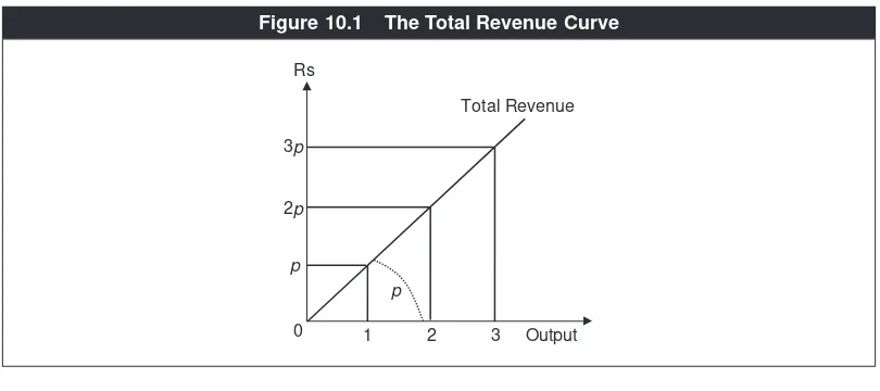
TR= price (p) ×quantity sold or produced (y).3Since pis given to the firm, its total revenue must equal p×1 if one unit is sold, p×2 if two units are sold and so on. Plotting these points against the output we obtain the total revenue curve, as shown in Figure 10.1. It is a ray from the origin with a slope equal to peverywhere because pis given to the firm.4A decrease or an increase in protates this curve clockwise or anti-clockwise respectively.
By now you might guess that with any ‘total’, there is always a ‘marginal’ and an ‘average’. This is true here. We define marginal revenue(MR) as addition to the total revenue from one extra unit produced and sold. In Figure 10.1 notice by how much TRincreases as one extra unit is produced. As output is increased from 0 to 1, MR= p−0 = p. Similarly, if output increases from 1 unit to 2 units, MR=2p−p= p. Thus, under perfect competition, MR=p. This is because pis exogenous to a firm.5 We now define average revenue (AR) as TR/output. Since TR=py, we have AR= py/y=p. Thus AR=p. Note that this has nothing to do with pbeing given to a firm. It holds in competitive and non-competitive markets.
As you will see shortly, it will be useful to have another graph called the price line, defined as a plot of price facing a competitive firm against its output. However, since p is exogenous to the firm it is simply a flat line as shown in Figure 10.2. From the price line we can measure the total revenue. If, for instance, the output = y1, TR=0p0×0y1=the area 0p0A1y1. Similarly at y=y2, the total rev-enue equals the area 0p0A2y2and so on. Hence, the (rectangular) area under the price line measures total revenue for a perfectly competitive firm.
Sometimes the price line is referred to as the ‘demand curve facing a competi-tive firm’ in the sense that irrespeccompeti-tive of how much a firm wants to sell or equiv-alently how much the consumers are buying from the firm, the price they are
Total Revenue
Output Rs
1 2 3
0
p
2p
3p
p
Figure 10.1 The Total Revenue Curve
3It is presumed that whatever quantity is produced is sold. There are no inventories.
4If the firm has any influence on the price, the total revenue curve will not be a straight line.
paying does not change.6We note that this demand curve facing a firm has price elasticity, equal to ∞.
PRODUCER’S EQUILIBRIUM IN THE SHORT RUN
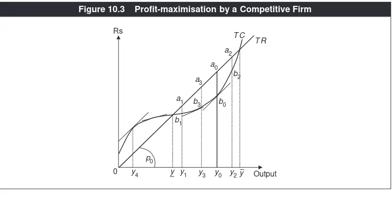
We are ready to analyse the profit-maximising behaviour of a competitive firm. Since profits are the difference between total revenue and total cost, one way to understand profit-maximisation is to look at the curves representing these in a single diagram as in Figure 10.3.
We can ‘read’ profits at any level of output. Notice that at outputs y
–and y–, the two curves intersect, implying that TR= TCand thus profits are zero. In other words,
Price Line Rs
Output
MR = AR
y2 A2 p0
0 y
1
A1
Figure 10.2 The Price Line
T C
Rs
Output
T R
p0
0 y4 y y1 y3 y0 y2y a2
a3 a0
b2
a1 b
3 b0
b1
Figure 10.3 Profit-maximisation by a Competitive Firm
6This is not, however, contrary to the law of demand, because here we are talking about the demand for the product by
these are the ‘break-even’ levels of output. If the output is less than y
– or greater thany–, TR< TCand hence profits are negative, that is, there are (abnormal) losses.
However, between y
– and y–, TR > TC and there are (abnormal) profits. Obviously, the firm would produce somewhere in this range. See Figure 10.3 and note that producing y3generates profit (equal to a3b3), which is higher than the profit (a1b1) associated with y1or the profit (a2b2) associated with output y2. But what is the level of output at which the profit is the maximum? Realise that it has to be the output y0at which the slope of the TRcurve (= the price p0) is equal to the slope of the TCcurve (= the marginal cost), that is, the tangent to the TCcurve is parallel to the TRline. Any output higher or less than y0yields less profit com-pared to y0. We can then say that profit is maximised at that level of output at which price equals marginal cost.
This condition does not, however, completely identify the profit-maximising output. Notice that, at the output y4also, the slope of the TRline is equal to the slope of the TCcurve, that is, p=MCholds. But, obviously, profit is not maximised at y4. Instead, there is a loss at this output. Apart from profit and loss, there is another difference between y4and y0—MC(the slope of the TCcurve) decreases with output around y4, while it increases with output around y0. This is the basis on which we can differentiate between y0 and y4, and identify the profit-maximising output y0. In general then, the profit-maximising output or the optimal outputof a competitive firm is characterised by the following conditions:
p=MC; MCis increasing in output. (8.1)
Often, the condition that MCis increasing is implicitly understood by economists and the profit-maximisation condition for a competitive firm is (loosely) stated as ‘p=MC’.
The economic reasoning behind the profit-maximising conditions (8.1) can be understood via Figure 10.4, which depicts the price line at p = p0, and a firm’s
MCcurve corresponding to the TRand TClines in Figure 10.3.
We see that p=MCholds at outputs y0and y4, which correspond to the same points in Figure 10.3. Around y4, MCis increasing, while around y0, it is decreas-ing in output. Applydecreas-ing economic reasondecreas-ing, we now argue that profit is
MC
Rs
Output 0 y4 y5 y′′ y′
p0
y0
maximised at y0, not at y4. Suppose that the firm is producing at y0. Consider an alternative of producing a slightly higher amount, say y’. Since MCis increasing, we see that MC > p
0. By definition, MC is the cost of producing the additional amount. Similarly, MR= pis the additional revenue. Thus, MC>p
0means that the additional cost is greater than the additional revenue. It implies that producing an amount slightly higher than y0yields less profit. Similarly, if the firm produced a bit less than y0, say y’’, MC<p
0. This holds also because MCis increasing in out-put around y0. That MC<p
0, as output is reduced from y0, means that savings in cost are less than revenues foregone. It is also a worse situation compared to pro-ducing at y0. This proves that around y0, producing y0yields maximum profit.
On the other hand, suppose the firm is producing at y4. Because MCis decreas-ing, if the firm produces a slightly higher amount (say y5), the market price would exceed MC, that is, extra revenue to be earned would be higher than extra cost to be incurred. This will bring more profits. Therefore, producing at y4 cannot be maximising profits. This completes the argument that out of the two output lev-els where p=MC, the profit-maximising one is where MCincreases with output.
Mathematically Speaking
Profit-maximisation by a Competitive Firm
A competitive firm’s total revenue has the expression, py. Let C(y) denote the total variable cost function and Fthe total fixed cost. Note that the marginal cost is the first derivative of the total variable cost function, equal to C’(y). Let C’’(y) denote the second derivative of the total variable cost function; if C’’(y) is positive (or neg-ative), the MCincreases (or decreases) with output. We can now express profits, π,
as the following function of y:
π =py−C(y) −F.
The firm chooses yso as to maximise π. The first-order condition of this
maximi-sation is:
(8.2)
This says that p=MC. The second-order condition is that d2π/dy2<0. (The
first-order and second-first-order conditions of unconstrained maximisation such as this is outlined in the General Appendix.) Totally differentiating dπ/dywith respect to y,
Thus, the second-order condition is met if and only
C’’(y) >0 (8.3)
(8.2) and (8.3) are indeed the conditions of profit-maximisation summarised in (8.1).
PROFITS, LOSSES AND THE SHUT-DOWN CONDITION
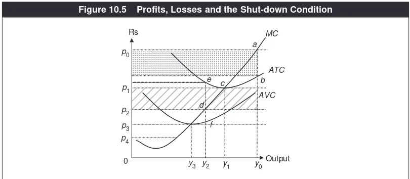
Profits and losses can be seen in a different diagram, which is quite useful. Turn to Figure 10.5, depicting various price lines and the firm’s MC, AVCand ATC curves. At price p0, the profit-maximising output is y0, as the MCat this output is equal to p0and the MCcurve is rising. The firm is making profits. The ATCis indi-cated as band the profit per unit of output, p−ATC, is the line segment ab. Total
profits are shown by the rectangular dotted area, equal to output times the profit per unit of output.
Consider next the price p1. The price line goes through the minimum point on the ATC curve, that is, p1 equals the minimum ATC. The optimal output is y1. Notice that at this output p=ATCand thus profits are zero; in the business
lan-guage, the firm is ‘breaking-even’. We can generally define break-even priceas that price at which profits are zero. The break-even price for a competitive firm is equal to the minimum ATC.
It is clear that at any price less than p1, the firm incurs losses. Consider p2, for example. The optimal output is y2. The ATCis indicated at the point eand ed meas-ures losses per unit. Total losses are shown by the rectangular shaded area. Similarly, you can calculate losses at the pricep3. They will be greater. At a further lower price such as p4, losses will be even greater than at p3.
A natural question arises here—should the firm not shut down (that is, produce nothing) if losses are being incurred? The answer is—not necessarily. Why? It is because in the short run the firm has to pay the fixed cost even if it decides not to produce any amount. For example, it has to pay the rent according to the lease agreement, repay loan to the bank and so on. In other words, shutting down does not mean that the profits are zero. It also involves a loss, equal to TFC. It is then pos-sible that by not shutting down, the firm’s losses are less as compared to shutting down. If the firm shuts down, its losses are TFC. Instead, if it operates (and produces
Rs
where p = MC), the losses are TC– TR= TFC– TVC– TR= TFC– AVC·y– py= TFC– (AVC– p)y. Therefore, the difference between the two levels of loss = (AVC– p)y. It then follows that the firm shuts down if p<AVC, that is, if the market price is less than the average variable cost at the profit-maximising output.7
It turns out that the above condition can be stated with more precision. Con-sider the particular price, which is equal to the minimum AVC. In Figure 10.5, this price is p3. Notice that at this price if the firm follows the p=MCrule, the optimal output is y3. Since at this output p=AVC, the firm should be indifferent between shutting down and not shutting down. It then follows that at any market price less than p3(equal to the minimum AVC), we have p<AVCand the firm should shut down. Therefore, we can state that at theShut-down Condition,
p<minimum AVC. (8.4)
NUMERICAL EXAMPLE 10.2
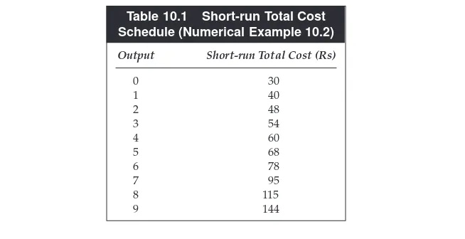
A competitive firm has a short-run total cost schedule as given in Table 10.1. What is the market price at which it will break even? What is the market price at which it will decide to shut down?
Dividing the total cost by output gives the ATC. See the level at which the output ATCis minimised. The minimised ATCitself is the break-even price. As we go down Table 10.1 from output equal to 1 to output equal to 8, the ATCs are respectively 40, 24, 18, 15, 13.6, 13, 13.85, 14.25 and 16. Hence the break-even price is Rs 13.
Next, note in particular that at zero output, the total cost is Rs 30. Hence, Rs 30 is the total fixed cost. If we deduct this from the total cost, we get the TVC. As we increase output, starting at 1, the TVCs are respectively equal to 10, 18, 24, 30, 38, 48, 65, 85 and 114. Dividing these by the respective outputs, AVCs are respectively equal to 10, 9, 8, 7.5, 7.6, 8, 9.27, 10.625 and 12.67. The minimum AVCis the price at which the firm will shut down and this is equal to Rs 7.5.
7If p = AVC, the firm is indifferent between shutting down and not shutting down. Table 10.1 Short-run Total Cost Schedule (Numerical Example 10.2)
Output Short-run Total Cost (Rs)
0 30
1 40
2 48
3 54
4 60
5 68
6 78
7 95
8 115
NUMERICAL EXAMPLE 10.3
Consider a competitive firm whose short-run total cost schedule is given in Table 10.1. The market price it faces is Rs 20. How much should it produce in order to maximise its profits? Is the firm making profits or incurring losses?
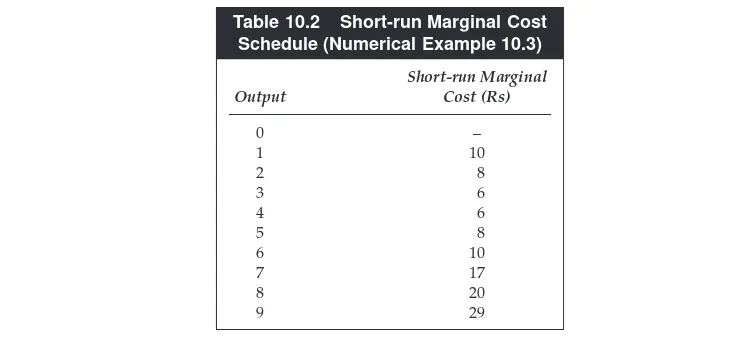
We first derive the marginal cost schedule from the total cost schedule. This is given in Table 10.2. The price = marginal cost condition is satisfied at output = 8. We also check that marginal cost is increasing around this level of output (it is 17 at output = 7, 20 at output = 8 and 20 at output = 9). Thus, profit is indeed maximised at output = 8. The maximised profit is equal to TR – TC = Rs 20 × 8 – Rs 115 = Rs 160 – Rs 115 = Rs 45.8
SHORT-RUN SUPPLY CURVE
Once we understand profit-maximisation and the shut-down behaviour, it is easy to derive the supply curve, introduced in Chapter 3. Recall that a firm’s supply curve is one showing the various quantities it is willing to produce and supply to the mar-ket at various prices, given technology and input prices. It is the counterpart of the demand curve in consumer theory. In consumer theory, the demand for a commod-ity was derived from the consumer’s optimal choice of the consumption bundle. Likewise, the supply curve is derived from the producer’s optimal choice of output. Turn back to Figure 10.5. If the market price is p0, we know that the profit-maximising output is y0, where p0= MC. Thus, y0is what the firm would supply to the market at price p0. The graph of this price-quantity pair is simply the point a. Similarly, at the price p1, the firm would supply the quantity y1and the
corre-8Another way to check whether the firm is making a profit or a loss is to compare the price with the break-even price. We already know from the Numerical Example 10.2 that the break-even price is Rs 13. Thus the market price is greater than the break-even price and, therefore, the firm must be making profits. Moreover, note that profit is maximised at output = 7 also. Two alternative answers arise because output is not measured on a continuous scale in this example—output only takes integer values, not decimals.
Table 10.2 Short-run Marginal Cost Schedule (Numerical Example 10.3)
Short-run Marginal
Output Cost (Rs)
0 –
1 10
2 8
3 6
4 6
5 8
6 10
7 17
8 20
sponding point on the MCcurve is c. The locus of points a, cand so on along the MCcurve is then the supply curve. However, not all the points on the MCcurve
would lie on the supply curve. We have just seen that the firm does not operate below the minimum AVC, which is also a point on the MCcurve. We can then say
that a firm’s short-run supply curve is its short-run marginal cost curve over and above the minimum AVCpoint. Since MCis rising, over and above the minimum AVCpoint on it, the supply curve is upward sloping. This is the economic
foun-dation behind the supply curve.
What factors can shift a firm’s supply curve? Since it is a part of the MCcurve,
whatever shifts the MC curve also shifts the supply curve. From what we have
learnt in Chapter 9 regarding the shift of the short-run MCcurve, it follows that a
technological improvement shifts the supply curve to the right, whereas an increase in an input price or in the rate of a business tax shifts the supply curve to the left.9
Time Horizon and the Market Period
Remember that we are considering a short-run period, meaning an interval of time during which a firm can vary some, but not all inputs.
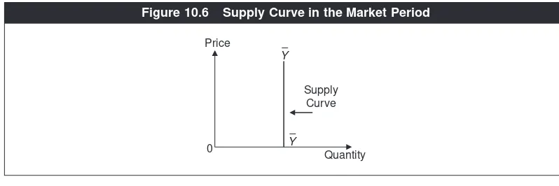
However, if the time period is very short, it is only natural that a firm cannot vary the employment of any input. Such a short period is called market period. How does the supply curve in a market period look like?
For instance, think of an agricultural good like paddy. It takes months between preparing the soil for the seeds and getting paddy ready for sale in the market during the spring season. How does the supply curve of paddy look like during the spring time? Given that it is already harvested and ready for sale, the quantity is fixed, irrespective of the price it is going to fetch. Accordingly, the supply curve for paddy during spring must look vertical, as shown in Figure 10.6, where Y–Y–is
the given quantity available for sale.
In sum, a period so short that no inputs and output can change is called market periodand the corresponding supply curve in the market period is vertical.
9From the individual, firm-level supply curves, the market supply curve is obtained by horizontally summing these. In Chapter 3, we have already discussed which factors shift the individual and market supply curves and how as well as the concept of price elasticity of supply.
Supply Curve Price
Y
0 Y
Quantity
Equilibrium in the Long Run
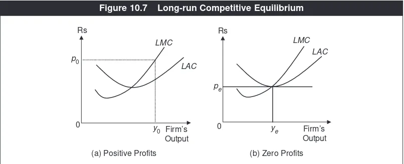
In the long run, when all—rather than some—inputs are variable, the profit-maximising behaviour of the firm remains qualitatively the same as in the short run. Profit is maximised at the output where the long-run marginal cost (LMC) is equal to the price and LMCis increasing in output. For instance, in Figure 10.7 that shows the LMCcurve and the LAC(long-run average cost) curve, if market price is p0, the firm produces y0 and there are abnormal profits. At pe, the firm pro-duces ye and the profits are zero. This is the break-even price, equal to the minimumLAC.
However, there is one important difference with the short run. Since there are no fixed costs, the firm would shut down—and leave the industry—as long as any loss is made. Why should a firm stay if it expects to lose in the long run? In view of Figure 10.7(b), we see that losses occur when price is less than pe. Hence, out-put or supply is zero as long as the price is less than the minimum average cost. This means that the long-run supply curve of a firm is the long-run marginal cost curve over and above the minimum long-run average cost point.
Comparison with the Short-run Supply Curve
Although both short-run and long-run supply curves are upward sloping, there is a qualitative difference between them (apart from that in terms of which part of the marginal cost curve they belong to). Recall that in the market period, no inputs can be varied and the supply curve is vertical. Over the short run, the firm has some flexibility, that is, some input level can be changed and the supply curve is upward sloping rather than vertical. Thus, the short-run supply curve is more elastic than the market-period supply curve. In the long run, the firm has even more flexibility as it can change the level of any input. Therefore, it can adjust its output more with respect to a change in the product price. Accordingly, the long-run supply curve is
Firm’s Output
0 Firm’s 0
Output
LMC
Rs
LAC
LAC
(a) Positive Profits (b) Zero Profits Rs
y0 ye
p0
pe LMC
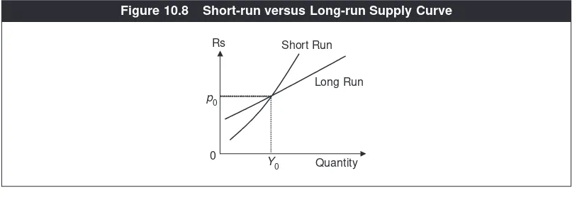
more elastic than the short-run supply curve.In terms of graph, it means that the long-run supply curve is flatter than the short-run supply curve.
This is illustrated in Figure 10.8. Suppose that initially in a long-run equilib-rium the firm was producing Y0 at price p0. If there is a price change from p0
(upward or downward), the output or supply adjustment is greater along the long-run than along the short-run supply curve.
Entry and Exit
Notice that free entry and exit is a characteristic of a perfectly competitive market and we have not said anything about it as yet. But it is relevant because in the long run, firms would like to enter into the industry or exit from it depending on whether they are earning (abnormal) profits or incurring (abnormal) losses. See Clip 10.1 for a newspaper article on how taxes have forced entrepreneurs in the movie-theatre industry to quit a market.
Industry equilibrium in terms of entry and exit is attained in the market when no firms have any incentive to enter or quit. This will happen when economic profits are zero. That is, entrepreneurs earn only their opportunity cost or what is called normal profit.
What is the zero-profit condition? We can write profit as (price – LAC) ×output. Thus, profits are zero if and only if price = LAC. Combining this with the profit-maximising condition of a firm, the overall firm-cum-industry equilibrium condi-tions are then:
Price =LMC=LAC. (8.5)
The firm-industry equilibrium is illustrated back in Figure 10.7, panel (b). The equi-librium price is pe, equal to the long-run minimum average cost, and the equilibrium firm-output is ye. We see that at this price-output combination, both the profit-maximising (price = MC) condition and the zero-profit (price = AC) condition are met.10Implicit here is that there is an equilibrium number of firms operating in the
10An important property of this long-run competitive equilibrium is that if we know the long-run average cost curve and
we know the long-run price of the product. In this sense, price is determined by technology only, not by demand—an observation made first by Alfred Marshall, who is regarded as the father of modern microeconomics.
Long Run Rs
Quantity Short Run
Y0
0
p0
market. Relative to market demand, too many firms would mean abnormal losses and too few firms would imply abnormal profits. A diagram such as Figure 10.7(b) cannot, however, show the equilibrium number of firms.
Realise that in the presence of entry and exit, an individual firm’s supply curve remains the same as before. But the nature of the industry supply curve— the horizontal sum of individual supply curves—is quite different because the number of firms in the industry changes in response to profits or losses being made. It is interesting that the long-run industry supply curve with free entry and exit of firms is a horizontal straight line (rather than an upward sloping curve). How is that?
Given the cost curves, we know the minimum LAC, say, equal to m.11Consider
the following possibilities. (i) Suppose the long-run market price is less than m.
Clip 10.1: 21 May 2005, Hindustan Times
Then no firm will be present in the industry in the long run; the industry output will be zero. (ii) Suppose the price is greater than m. New firms will keep entering and thus the industry output will be arbitrarily large. In the language of mathe-matics, it is infinity (∞). (iii) If the price is exactly equal to m,the industry output
is indeterminate from the supply side. Of course, in the last case, the equilibrium quantity supplied to the market must equal the quantity demanded along the market demand at the price equal to m.
By combining the possibilities (i), (ii) and (iii), the industry supply curve is then a horizontal line whose height is equal to the minimum LAC, as shown in Figure 10.9.
The practical implication of such long-run equilibrium with free entry and exit is that the price is driven down to its unit cost. Note that the unit cost of a prod-uct depends, in part, on technology. Thus, in the long run, the price of a prodprod-uct is essentially dictated by its technology—an important remark made, a long time ago, by Alfred Marshall.
A good example of competition driving down the price to the unit cost as firms enter and leave the industry is the personal computer market. The technology is so standard that assembling a computer takes no more than an hour and loading software is no more than a two–three-hour job. Entering this business and getting out of it are rather easy. As you can look around and see, there are many computer vendors in the market in most parts of India. You ask any vendor today about how much profit they make per unit sold. The business is so competitive that it is no more than Rs 1,000.
However, in some other businesses, the entry and exit processes are costly and time consuming. In the old era of licence raj, to start any major business one was supposed to obtain a licence and a number of clearances from the government. Any experienced, aged entrepreneur will tell you how painful it was to obtain these permissions in terms of crossing numerous layers of bureaucracy, corruption and delay. However, in the post-liberalisation era, it is a much simpler process (yet, in comparison to many other countries, still very costly).
Of course, getting a licence may be just one deterrent for entry into a business. Another may be the initial capital needed to set up a plant and getting production
Min LAC
Price
Industry Supply Curve with Free Entry and Exit
Industry Output 0
going. When the technology is such that the initial capital requirement is huge, it works as a natural deterrent to entry. Typically, in these industries those who are able to enter and survive earn abnormal profits over a long period of time (as it is hard for others to enter).
NUMERICAL EXAMPLE 10.4
A competitive industry has many identical firms. Each firm’s long-run marginal cost schedule is given in Table 10.3. The market demand schedule for the product is given in Table 10.4. In the long-run equilibrium, how many firms would oper-ate in this industry?
From the long-run marginal cost schedule, we can derive the long-run total cost schedule by adding up marginal costs. From the latter, we can derive the
long-run average schedule through dividing the total cost by output. The LAC
schedule is given in Table 10.5. We notice that this is minimised at output = 4. Hence, in the long-run equilibrium, each firm produces 4 units. The (minimised)
LAC= Rs 8.5; this is the long-run market price as in the long-run equilibrium, the
market price is equal to the minimum LAC. We now utilise Table 10.4. At price =
Rs 8.5, 40 units are demanded. In equilibrium, 440 units are produced in the industry. Since each firm produces 4 units, the number of firms in operation must be equal to 440/4 = 110.
Table 10.3 Long-run Marginal Cost Schedule (Numerical Example 10.4)
Output LMC
1 10
2 9
3 8
4 7
5 9
6 11
7 12
Table 10.4 Market Demand Schedule (Numerical Example 10.4)
Price Quantity
Rs Demanded
5.5 468
6 465
7.5 460
8 450
8.5 440
9 420
Economic Facts and Insights
● Economic analysis and decision-making take into account economic profit,
not accounting profit.
● The product being homogeneous and the industry being populated with a
large number of firms implies that an individual firm is a price taker in a competitive market. It means that no single firm has any market power.
● A perfectly competitive firm maximises profits by producing at a level of
output such that the market price equals marginal cost and marginal cost is increasing in output.
● In the short run, a firm may be making profits or incurring losses.
● Even if a firm is making losses in the short run, it should not necessarily shut
down (because the firm has to pay the fixed cost whether or not it shuts down).
● The supply curve of a competitive firm is a part of its marginal cost curve.
● In the market period, the supply of a product is fixed.
● The long-run supply curve is more price elastic than the short-run supply
curve of a firm.
● In the long run, with free entry and exit, firms make zero or normal profit.
● The long-run firm-cum-industry equilibrium is characterised by the market
price being equal to the long-run marginal cost as well as the long-run aver-age cost.
● The long-run industry supply curve with free entry and exit is a horizontal
straight line.
● In the long-run competitive equilibrium, the price of a product is essentially
governed by its technology.
Table 10.5 Long-run Average Cost Schedule (Numerical Example 10.4)
Output LAC
1 10
2 9.5
3 9
4 8.5
5 8.6
6 9
