Essays in Macroeconomic Models with Financial Frictions By
Frank A. Ciarliero
Dissertation
Submitted to the Faculty of the Graduate School of Vanderbilt University
in partial fulfillment of the requirements for the degree of
DOCTOR OF PHILOSOPHY in
Economics
August 7th, 2020 Nashville, TN
Approved:
Peter L. Rousseau, Ph.D.
Mario J. Crucini, Ph.D.
Robert A. Driskill, Ph.D.
Kevin X. D. Huang, Ph.D.
David C. Parsley, Ph.D.
for the First Peoples of the continent of Australia...
ACKNOWLEDGMENTS
The completion of this dissertation is the culmination of many years of education at all the possible levels. I extend my gratitude to all the educators who have taught and nurtured me throughout.
I thank my advisor Peter Rousseau for comments and helpful guidance throughout my years in graduate school. Above all, his belief in my abilities and talents has inspired me to reach the finish line.
I recognize the assistance of Vanderbilt University in providing supporting funds throughout my tenure here. In particular, enrolling in this program has allowed me to learn from my committee members Mario Crucini, Robert Driskill (who I am implored to call Bob), Kevin Huang, and David Parsley, at various stages, both in research and in the classroom. I profoundly thank them.
Beyond my committee, I thank the other faculty members who guided me in various ways throughout and presented me with opportunities, particularly Eric Bond, Greg Huffman, Greg Leo, Kathleen McKiernan, Hyunseung Oh, Joel Rodrigue, and John Weymark. Special thanks to Kathleen Finn, whose kindness personifies the pleasant time I have had in Nashville.
I have met many wonderful and diverse classmates in the Vandy economics graduate cohort.
To my perennial office mates Nicolas M¨ader and Zeeshan Samad, along with Caroline Abraham, Daniel Mangrum, Paul Niekamp, Oscar O’Flaherty, and Jonah Yuen, I say thanks for being great friends.
Above all, I thank my family and wonderful partner Rebekah Austin. The greatest contribution they made among many, was providing the implicit knowledge that irrespective of the outcome of my brash choice to move to the United States or the outcome of this research, that I would be loved unconditionally.
TABLE OF CONTENTS
Page
DEDICATION . . . ii
ACKNOWLEDGMENTS . . . iii
LIST OF TABLES . . . vi
LIST OF FIGURES . . . vii
LIST OF ABBREVIATIONS AND NOMENCLATURE . . . viii
Chapter Introduction . . . 1
I. Money on the Sidelines? The Role of Costly Search and Weak Loan De- mand in the Slow Recovery . . . 3
1. Introduction . . . 3
2. Stylized Facts from Key Financial Aggregates . . . 8
3. The Market for Loans to Non-Financial Firms . . . 12
3.1. Search and Matching . . . 13
3.2. Interest Rate Bargaining . . . 16
4. The Model . . . 18
4.1. Households . . . 18
4.2. Firms . . . 21
4.3. Banks . . . 26
4.4. Government . . . 29
5. Data and Variable Construction . . . 31
6. Results . . . 36
6.1. Parameter Estimates . . . 37
6.2. Impulse Response Functions . . . 42
6.3. Estimated Shocks . . . 47
6.4. Variance Decompositions . . . 49
6.5. Model Fit . . . 51
7. Conclusion . . . 52
II. Investment on the Extensive Margin. Replacement, Maintenance, and the Role of Credit. . . 54
1. Introduction . . . 54
2. The Model . . . 57
2.1. Capital . . . 57
2.2. Credit Cards . . . 58
2.3. Bankruptcy . . . 59
2.4. Value Functions . . . 59
2.5. Aggregation . . . 62
2.6. Calibration . . . 63
3. Results . . . 65
3.1. Policy Functions . . . 65
3.2. Simulations . . . 69
4. Conclusion . . . 75
III. Velocity Targeting at the Zero Lower Bound . . . 77
1. Introduction . . . 77
2. The Model . . . 79
2.1. Derivation of theClarida, Gal´ı and Gertler (2000) Rule . . . 79
2.2. Derivation of Target Money Velocity . . . 80
3. Data and Estimation . . . 83
3.1. Structural Regression Model . . . 83
3.2. Data . . . 85
4. Results . . . 87
5. Conclusion . . . 91
REFERENCES . . . 92
APPENDICES . . . 97
A.1. Appendix for Chapter I . . . 97
A.1. Data Construction . . . 97
A.2. Technical . . . 99
A.3. Other Impulse Response Functions . . . 111
A.2. Appendix for Chapter II . . . 116
A.1. The Model ofCooper, Haltiwanger and Power (1999) . . . 116
A.2. Solution Method . . . 116
LIST OF TABLES
Table Page
1. Cyclical Relationships of Bank Balance Sheet Aggregates . . . 10
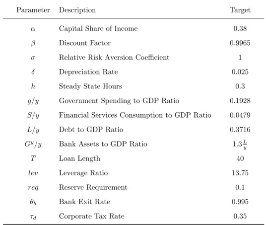
2. Calibrated Parameters and Steady State Targets . . . 36
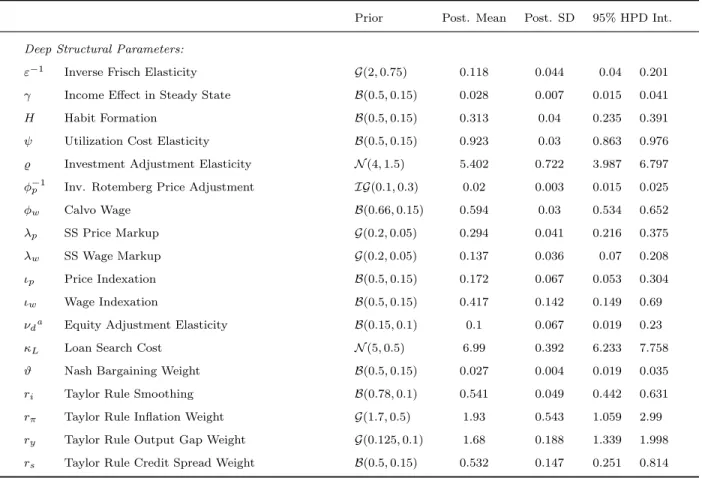
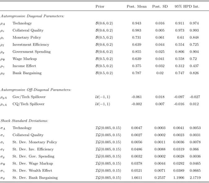
3. Bayesian Parameter Estimates . . . 38
3. Bayesian Parameter Estimates . . . 39
4. Variance Decomposition . . . 50
5. Model Fit Measures . . . 51
6. Summary of Discrete Choices Available to Firms . . . 60
7. Calibrated Parameters . . . 64
8. Long-Term Aggregate Ratios in Simulations . . . 73
9. Interest Rate Inertia Estimation . . . 88
10. Regression Results for Velocity Autoregressive Process . . . 90
A.1. Sources of Raw Data . . . 97
A.2. Construction of Estimation Variables . . . 98
A.3. Construction of Variables Used for Calibration . . . 98
LIST OF FIGURES
Figure Page
1. Assets in Aggregate US Banks’ Balance Sheet . . . 9
2. Senior Loan Officer Opinion Survey on Bank Lending Practices . . . 11
3. Interest Rates by Risk Level . . . 12
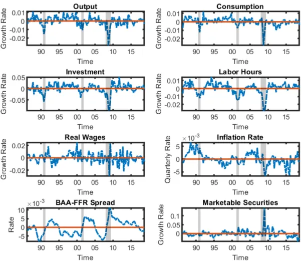
4. De-meaned Time Series Used in Estimation . . . 33
5. Impulse Responses—Technology Shocks . . . 43
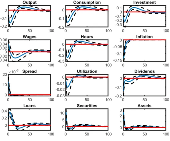
6. Impulse Responses—Investment Efficiency Shocks . . . 45
7. Impulse Responses—Monetary Policy Shocks . . . 46
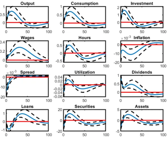
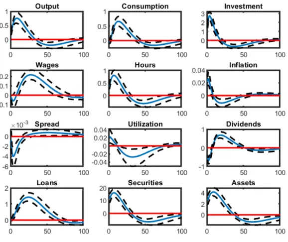
8. Impulse Responses—Collateral Quality Shocks . . . 47
9. Estimated Shocks . . . 48
10. Investment Policy Function . . . 66
11. Repayment Policy Function . . . 67
12. Forbearance and Bankruptcy Policy Functions . . . 69
13. Simulation of a Single Firm . . . 70
14. Simulation of at the Industry-Level . . . 71
15. Model Comparison . . . 73
16. Effective Vintage Distribution . . . 74
17. Actual Vintage Distribution . . . 75
18. Aggregate Data . . . 86
19. M1 Velocity . . . 87
20. Actual vs Fitted Interest Rate Values . . . 89
A.1. Impulse Responses—Government Spending Shocks . . . 112
A.2. Impulse Responses—Bank Bargaining Weight Shocks . . . 113
A.3. Impulse Responses—Wage Markup/Labor Disutility Shocks . . . 114
A.4. Impulse Responses—Income Effect in Labor Supply Shocks . . . 115
LIST OF ABBREVIATIONS AND NOMENCLATURE
Aaa Bond Moody’s investment grade rating for corporate and sovereign debt.
Baa Bond Moody’s junk grade rating for corporate and sovereign debt.
Capital Structure The mix of debt and equity a firm employs to finance its operations.
DSGE Dynamic Stochastic General Equilibrium Model
Extensive Margin A decision taken whereby the choice is between undertaking an activity or not.
GDP Gross Domestic Product
GMM Generalized Method of Moments
Inflation The rise in prices from period to period.
Intensive Margin A decision taken whereby the intensity of an activity is chosen.
Quantitative Easing Monetary Policy conducted to target long-term interest rates and im- plemented via bond purchases.
INTRODUCTION
This dissertation explores the consequences, or lack thereof, of the presence of financial frictions in micro-founded models of the macroeconomy of the United States (US) and in the practice of monetary policy by the Federal Reserve. I primarily explore the effects of different types of firm borrowing, focusing on long-term collateralized debt in Chapter I and its general equilibrium effects where household, firm, and banking decisions are made on the intensive margin. In Chapter II, I specifically consider extensive margin decisions and how they are affected by a debt structure that is unsecured. Chapter III offers an exploration of US Monetary Policy following the Great Recession. In this time period, overnight rates were held for many years at the zero lower bound and questions arose regarding central bankers’ ability to pursue their policy objectives.
The research illuminates the specific transmission mechanisms in the economy of policy changes and aggregate shocks when financial frictions are present and modeled in a structural manner.
Moreover, I shed light on which time series in the data carry identification power for these underlying shocks.
In Chapter I, firms and banks search for counterparts to execute long-term loan contracts with.
I find that financial shocks to the collateral quality of existing capital create incentives in the firm to increase investment so that they may maintain their desired capital structure. The general equilibrium effects into household balance sheets from this behavior occur via wealth effects, sub- stantially depressing consumption in financial recessions, boosting work incentives, and depressing real wages. The series of bank marketable securities provides the identification power that allows us to distinguish a recession that originates in the financial as opposed to the productive sector of the economy. I model marketable securities as an outlet for banks to invest funds in that could otherwise be directed to lending. The timing of increases in this series sheds light on the underly- ing state of the economy. An increase in marketable securities absent a wider economic slowdown suggests a relative withdrawal of lending liquidity by banks; a financial recession. In contrast, when marketable securities rise following a wider productive downturn, we recognize a lack of demand for funds from the private sector. This suggests a recession with its genesis in the real sector.
While Chapter I features intensive margin decisions being made by the economic agents, a substantial body of work demonstrates that many, and possibly all, crucial firm decisions are made on the extensive margin. Chapter II delves into models of lumpy investment. Models which to date have captured the firm-level dynamics quite well, but not necessarily aggregate dynamics.
By adding an element of financial frictions via revolving debt, I am able to induce investment substitution along the extensive margin. Firms elect to replace capital, a large investment outlay, in a strong aggregate state of the economy, and when financial conditions are conducive. When debt funding capacity is lacking, firms substitute to relatively more modest maintenance investment.
The operation of this maintenance channel allows the enhanced lumpy investment model to exhibit more accurate aggregate properties and also improves the model’s fit at the firm-level.
In terms of policy implications, the results in Chapter I allow policymakers to better target their responses as a result of being able to discern the underlying cause of any downturn in real time. Arising in Chapter II are potentially new implications for stimulating investment. Aggregate investment is highly path dependent in the model, with replacement investment responding strongly in volatile periods. Long periods of aggregate stability can lead firms to enter an apparent stasis where most investment outlays are in the form of maintenance. This is an insight that should be taken into consideration.
Chapter III considers an institutionally induced financial friction, the zero lower bound on nominal interest rates. A debate has emerged following the Great Recession with one side viewing monetary policy as constrained by the zero lower bound in the time period ensuing. The competing view is that the Federal Reserve has been able to implement its goals via alternate means. The results in this chapter support the latter viewpoint. I specifically find that the zero lower bound was binding as a constraint in the post Great Recession period. However, this did not limit the ability of central bankers to achieve their price stability and full employment mandate. Rather, the Federal Reserve was able to pivot towards a practice that effectively targeted money velocity, implementing its implied policy stance therein.
The following dissertation elucidates the above in greater detail, describing the modeling ap- proaches and innovations, and detailing the empirical methodologies employed.
CHAPTER I
Money on the Sidelines? The Role of Costly Search and Weak Loan Demand in the Slow Recovery
1. Introduction
The financial crisis that triggered the Great Recession saw sizable reductions in the depth of credit markets. The provision of loans fell sharply while credit spreads widened, making the experience seem like a financial supply shock. The policy response was unconventional, with the Federal Reserve directing generous sums of liquid funds to banks. Banks were well capitalized following successful rounds of capital raising and laden with funds, yet lending was subdued. This is known colloquially as ‘money on the sidelines’, a phrasing which suggests a lack of willingness to lend by banks. Rather than accepting that interpretation, this paper develops an endogenous channel where new frictions in loan markets allow for the identification of periods of weak loan demand as distinct from a financial crisis where loan supply is reduced.
The Great Recession was sizable with a longer duration than other downturns in the post World War II experience, coupled with a particularly slow recovery. This is a peculiar happenstance in the context of existing models and the practice of unconventional monetary policy during and following the crisis. The expectation would be that a large injection of funds to banks would flow quickly as loans to firms and stimulate economic activity. However, the lived experience was that bank credit to the private sector fell dramatically just as liquid bank assets were growing strongly.
In particular, this growth was seen in excess reserves, suggesting a gap in existing models that neglect to define channels whereby banks can invest available funds rather than loaning them. The policy implications are stark. A government authority seeking to alleviate the recession and quicken the pace of recovery should not only concern itself with the provision of funds to banks, but also their dissemination as loans. The evidence in this paper suggests that policy during the recession successfully restored financial markets quickly but neglected the private sector, which by the latter part of the crisis and into the recovery phase saw firms reducing their loan demand due to a lack
of available investment avenues.
As conjectured in Kashyap and Zingales (2010), meaningful financial spillovers of the type motivated by the experience of the Great Recession are not possible when debt adjustment is cost- less.1 In this paper, capital structure decisions are non-neutral and result in a productive cost to adjusting the debt to equity mix for firms. The first source of non-neutrality is an intermediation friction in loan markets that I model with a search and matching approach. Secondly, loans are repaid over multiple periods according to an annuity formulation.2 This has the effect of front loading the weight of the interest component of any repayment, making the firm more susceptible to adverse changes in interest rates following large loan acquisitions.
This loan market is embedded in the workhorse New Keynesian model with loans being supplied from leverage ratio optimizing banks.3 Costly search for long-term loans leads to an endogenous term structure arising from the model. Such a channel expands the empirical reach of DSGE models, allowing us to account for the counter-cyclically widening credit spread observed in the data, which was a prescient feature of the Great Recession.
Additionally, imperfect matching in the loan market endogenously generates distinct categories of bank assets. Successful matching results in the creation of a loan, while a failure to match forces banks to divert available funds towards marketable securities. This feature allows the model to account for the build-up of marketable securities seen in the Great Recession and to a lesser extent in recessions prior. Two competing forces can account for increasing marketable securities in this setup. Either firms reduce loan search or banks withdraw some leverage. Both have the effect of inducing less loan matching, however, whether this is a demand or supply driven phenomenon is critical in deciding the appropriate policy response.
The key identifying relationship in the model with the addition of the long-term loan market is the cyclical behavior of investment. As opposed to standard treatments where investment is strongly pro-cyclical in response to all shocks, firm behavior in this model sees investment responding most when the investment-specific environment is strong. This is the case of an investment efficiency
1New Keynesian models such as Christiano, Eichenbaum and Evans (2005), Smets and Wouters (2007), and Justiniano, Primiceri and Tambalotti(2011), implicitly assume that real aggregates are invariant to capital structure decisions.
2SeeAlpanda and Zubairy(2017) andQuint and Rabanal(2017) for works that feature long-term loans in other macroeconomic contexts.
3I use the structure ofGertler and Karadi(2011) to model bank behavior.
shock. Here, the firm requires financing for its investment, building up loans slowly and meeting any shortfall with equity. In contrast, in response to a positive financial shock, the firm will bias its behavior toward loan search, taking advantage of looser lending standards to finance itself with relatively more debt than equity. Here, investment is allowed to drift, exhibiting short-term counter-cyclical behavior.
That the model produces these distinct investment paths is crucial to its micro-foundational validity. In times when the investment response is subdued, so too is the response of its price, the risk-free real interest rate. As a result, positive shocks do not necessarily induce household saving behavior, which normally require a strong labor hours response to wage changes to produce the coincidentally pro-cyclical pattern of output, consumption, investment, and labor hours movement seen in the data. In contrast, the channel in this paper is a strong household wealth effect stem- ming from household ownership of firms that substitute to equity financing when debt demand is unsatisfied in the short-term.
The spillover of loan decisions into productive outcomes places this paper in the class of models that contain financial frictions.4 The theoretical contribution of this paper in this context is to explore the interplay between banks and firms in general equilibrium, capturing the disaggregated bank asset reallocations between loans and marketable securities. These additions are embedded in the existing framework, allowing the model to exhibit the empirically observed co-movements concurrently across real and financial variables.
The augmented model is estimated via Bayesian methods, utilizing an expanded set of observ- ables that additionally include a measure of aggregate marketable securities held by banks and a measure of the credit spread. This approach facilitates an empirical evaluation of the model on the supply and demand sides of the real economy, labor market, and newly in this chapter, the loan functions of banks in the US economy. The simulation at the posterior mean provides a rich business cycle narrative of the post-Volcker period of the US economy. The 1991 and 2001 reces- sions were both caused by a combination of monetary policy, technology, and investment efficiency shocks. Quite distinctly, the Great Recession is financial in nature at the onset, becoming a real
4See Bernanke, Gertler and Gilchrist (1999) and Kiyotaki and Moore (1997), for early incarnations of such models, with Ajello (2016), Akinci and Queralto (2016), Bigio (2015), Christiano, Motto and Rostagno (2014), Gertler, Kiyotaki and Prestipino(2018),Gomes, Jermann and Schmid(2016),Jermann and Quadrini(2012),Nu˜no and Thomas(2017) being recent examples of general equilibrium developments in financial frictions macroeconomic models.
recession caused by a weak investment environment during its second phase. Moreover, the sim- ulated shock series exhibits rising aggregate productivity during the Great Recession, consistent withAnzoategui et al. (2019), who show such technology movement.5
Under the propagation mechanism of the model, a period of weak investment-specific produc- tivity would produce subdued loan demand from firms. This is consistent with micro-level surveys of senior loan officers in US banks, who reported decreased demand for loans in the latter part of the recession. The other main finding in that survey is the reporting of tightening lending standards in the first half of the crisis, which the model captures via a negative financial shock.
In addition to examining the model for its adherence with micro-evidence, I also assess the parameter fit and likelihood. Can the model implied simulation of the observed time series match the data for plausible parameter values? Does the model fit the data at the posterior mean with a high likelihood? Unfortunately, employing an expanded set of observables that extend beyond the scope of the basic New Keynesian model renders it impossible to perform a comparison of model likelihoods. On the other hand, the question of reasonable parameter estimates can be addressed.
Following Bayesian estimation, the parameter estimates broadly conform with existing studies in investment and capital utilization adjustment costs, however, the model requires substantially lower levels of nominal frictions and habit formation to generate the observed data.6 This is a desirable outcome because many of those frictions are considered to be of dubious grounding at the microeconomic level. Additionally, the Frisch elasticity of labor supply is estimated to be higher than seen in typical studies, which reflects recent contributions concerning the interpretation of labor supply made inChristiano, Trabandt and Walentin (2011).
Having estimated the model, I then turn to the question of addressing the extent to which each shock explains the US business cycle. By way of variance decomposition at different horizons, I find that investment efficiency and technology shocks account for the majority of the US business cycle at long-term horizons. However, financial shocks captured by a fall in the value of existing capital as collateral, account for the majority of short-term business cycle fluctuations. That
5The results hold whether technology is measured by labor productivity or capacity-adjusted total factor produc- tivity.
6New Keynesian DSGE models feature habit formation in consumption, sticky prices and wages, wage and price indexation, costly investment adjustment, and costly capital utilization adjustment to fit the data. SeeChristiano, Eichenbaum and Trabandt(2016) for a survey of the micro-level evidence of the plausibility of some of these frictions.
More recent work byKeen and Koenig (2018) explores the plausibility of wage and price indexation, whileChetty and Szeidl(2016) explores habit formation.
result is indicative of the role of financial frictions in firm-level behavior. Short-term denials of financing severely dampen a firm’s productive capabilities. In the long-run, the ideal debt position becomes attainable, and business cycle fluctuations are the result of persistent shifts in productivity, particularly of new investment.
Beyond the contribution to the US business cycle literature, I address criticisms in Chari, Kehoe and McGrattan (2008) and Canova and Sala (2009) that question the exogeneity of shocks to the price markup and risk premium. These shocks potentially capture endogenous shifts in competition and also ‘flight-to-quality’ responses, respectively. This critique is not trivial, with their inclusion potentially biasing parameter estimates and limiting identification. To overcome these issues, I utilize alternative shocks in the model that allow me to continue to include the full set of observables used in prior studies, while continuing to identify all parameters and shock series.7
Specifically, I assume exogenous variation to the parameterized wealth effect of real wage shifts, and a Nash bargaining weight that captures the relative importance of banking competition or intermediation costs in determining the credit spread. The former of these is a deep preference parameter for which to my knowledge, there is no evidence of endogenous variation. The second shock is potentially deficient in the same manner as the excluded types. For this to be the case, the business cycle would need to endogenously affect the cost of bank intermediation or the level of bank competition. The latter is unlikely as banking merger and acquisition activity is highly regulated, and the implicit existence of ‘too-big-to-fail’ type policies render network wide banking failures unlikely. However, intermediation costs do plausibly suffer from endogeneity issues. The view taken in this paper then is that the inclusion of these two new shocks leads to no worse an outcome than the standard estimation approach, and perhaps an improvement. The paper serves to illuminate the possibilities of utilizing alternate shocks.
The endogenous generation of a credit spread in the model allows the paper to make a policy contribution. Specifically, credit spreads can be added to the standard Taylor Rule as suggested by C´urdia and Woodford (2016), and as empirically supported in the post recession period by
7The other alternatives to including potentially endogenous shocks is to estimate the model with fewer observed time series, limiting and sometimes eliminating identification of some parameters. Alternatively, measurement errors can be included in the measurement equations that map the model variables to their data counterparts. This approach is problematic where such errors are not warranted by the data. SeeCanova, Ferroni and Matthes (2014) for a full analysis of these issues. Cuba-Borda et al.(Forthcoming) expand upon other issues with measurement error use.
Caldara and Herbst(2019).8 I include such an augmented rule in the model and assign a partially informative prior to the Taylor Rule weight on the credit spread. In particular, the prior is slightly biased towards the range of values that suggest little or no monetary policy response to credit spreads. Following estimation, the posterior distribution drifts away from the prior mean and towards the range of values implying monetary intervention following credit spread shifts.
The remainder of this paper is organized as follows, Section 2 provides greater detail about the aforementioned stylized facts that are utilized in estimation. Section 3 describes the structure of the loan market. Section 4 describes the model and optimization problems for each of the agents, as well as the specification of monetary and fiscal policy. Section 5 describes the data and variable construction used in the Bayesian estimation. Section 6 presents the results, and Section 7 concludes.
2. Stylized Facts from Key Financial Aggregates
The key empirical regularity that is exploited in this paper is bank substitution between loans to the private sector and marketable securities. Loans to the private sector (Loans) is defined herein as the sum of the value owed to banks from lending contracts with a borrowing counter-party. In contrast, marketable securities are the sum of the value of all assets held that are tradeable, making these liquid assets. They can be excess cash that are not a part of required reserves, loans to other banks, and holdings of treasury and mortgage backed (MBS) securities. The balance sheet identity for banks on the assets side is,
Assets=Loans+M arketable Securities+Required Reserves
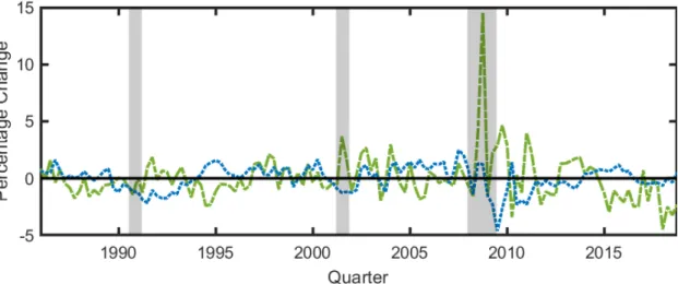
All bank assets are loans or required reserves at the aggregate level, however, Figure 1 demon- strates a clear distinction in the cyclical behavior of the disaggregated component parts. Marketable securities are starkly counter-cyclical, particularly during the Great Recession, and to a lesser extent in the other two recessionary episodes. Loans experience periods of growth during non-recessionary periods. Moreover, this growth occurs with a substantial lag following recessions.
8The standard Taylor Rule is assumed to follow the specification empirically observed inClarida, Gal´ı and Gertler (2000).
*Source: Federal Reserve Board of Governors Release H.8 Assets and Liabilities of Commercial Banks in the United States. Quarterly data from 1986 Q1 to 2019 Q1. ∆M Sis the growth rate of log per-capita real marketable securities, where marketable securities is the sum of bank holdings of treasury and mortgage-backed securities, cash, loans to other banks, and other assets, less required reserves. ∆Lis the quarterly growth rate of log per-capita real loans and leases in bank credit.
Both series are de-meaned.
Figure 1. Assets in Aggregate US Banks’ Balance Sheet
Table 1 shows that the growth rates of marketable securities and loans are more volatile than real GDP, with marketable securities representing the most volatile series. Also, while marketable securities growth is most negatively correlated with GDP growth contemporaneously, loans are most positively correlated with GDP at a lag of eight quarters. Additionally, marketable securities and loans are negatively correlated, and this is strongest for eight quarter lags of marketable securities.
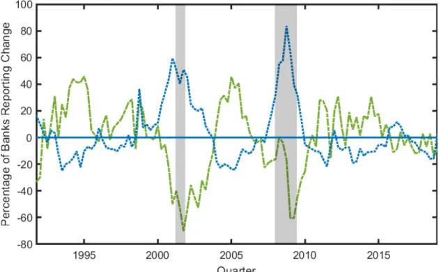
Figure 2 gives us an indication as to the micro-level behavior underlying the cyclical movement of loans and marketable securities. Senior loan officers are asked to report whether their bank (i) raised lending standards and (ii) faced stronger loan demand. The movement of these series displays a striking resemblance to the aggregate movements of the two categories of bank assets, suggesting that a model that features a channel for firms to vary their loan demand and for banks to change lending standards could reconcile the co-movement of real and financial aggregates. Moreover, the differences in the senior loan officer responses across the two recessionary periods sheds light on the financial conditions of the economy during both periods. In 2001, standards and demand exhibit near perfect negative correlation. In contrast, in the Great Recession, standards are first rising
Table 1. Cyclical Relationships of Bank Balance Sheet Aggregates
x St. Dev. Corr(x,∆GDP) Corr(x,∆GDP−8) Corr(x,∆M S) Corr(x,∆M S−8)
∆GDP 0.0057 1 -0.0583 -0.2155 -0.0549
∆M S 0.0203 -0.2155 -0.1051 1 -0.0682
∆L 0.0111 0.0112 0.2815 -0.073 -0.1555
*Source: Federal Reserve Board of Governors Release H.8 Assets and Liabilities of Commercial Banks in the United States. Quarterly data from 1986 Q1 to 2019 Q1. ∆M S is the quarterly growth rate of de-meaned log per-capita real marketable securities, where marketable securities is the sum of bank holdings of treasury and mortgage-backed securities, cash, loans to other banks, and other assets, less required reserves. ∆Lis the quarterly growth rate of de-meaned log per-capita real loans and leases in bank credit.
**Source: US Bureau of Economic Analysis National Income and Product Accounts. Quarterly data from 1986 Q1 to 2019 Q1. ∆GDP is the quarterly growth rate of de-meaned log per-capita real GDP.
in the middle part of the recession while demand is not changing, suggesting a specific financial shock. Demand is then starkly weaker for two consecutive quarters while standards were beginning to moderate. The results in this paper suggest that the late recession fall in loan demand is the result of an investment-specific shock that follows a financial shock, rather than a response to banks withholding funds due to tighter standards alone.
We seek a modeling structure that is able to incorporate these stylized facts in the financial sector of the economy, while continuing to capture the extensively documented standard business cycle stylized facts on the real side of the economy. Search and matching frictions that incorporate costly loan search are appealing. Such a structure endogenously prevents banks from loaning all available funds, reflects information asymmetries inherent in the loan market by way of a reduced form matching function, and allows for the slow accumulation of loans, as not all requests for financing are immediately satisfied.
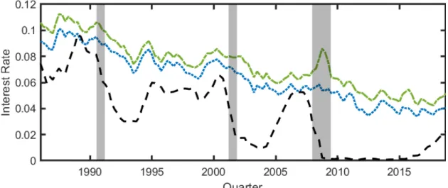
The second prescient stylized fact motivating this paper is the evolution of interest rates and credit spreads over the cycle. The Great Recession is distinct to the others in that the Baa corporate bond rate moves counter-cyclically while the federal funds rate is adjusting in a highly cyclical manner. This effect appears to be related to the underlying riskiness of such loans, with the Aaa rate remaining relatively flat in contrast.
*Source: Federal Reserve Board of Governors Senior Loan Officer Opinion Survey on Bank Lending Practices. Quarterly data from 1991 Q4 to 2019 Q1. Series are (i) Net Percentage of Banks Reporting Stronger Demand for Commercial and Industrial Loans for Large and Middle-Market Firms, (ii) Net Percentage of Banks Reporting Tightening Standards for Commercial and Industrial Loans to Large and Middle-Market Firms.
Figure 2. Senior Loan Officer Opinion Survey on Bank Lending Practices
Under the search and matching structure, interest rate and quantity determination are decou- pled. A Nash bargaining surplus sharing rule will instead determine the interest rate. This modeling choice allows for distinct channels that can capture the interest rate dynamics and movements in the quantity aggregates. That interest rates do not clear the loan market is not a novel concept, beginning with Stiglitz and Weiss (1981) where credit rationing is the channel through which the loan market clears.
*Source: Board of Governors of the Federal Reserve System. Quarterly average of monthly rates.
Units are annualized.
Figure 3. Interest Rates by Risk Level
3. The Market for Loans to Non-Financial Firms
Before commencing with a description of the loan market, it is useful to first consider why firms would hold an outstanding amount of debt at all. Most closed economy representative agent models have the feature that there is no net aggregate debt holding in equilibrium.9 Alternatively, non-zero levels of bond holdings in equilibrium can be induced by assuming some heterogeneity in levels of patience among different agents. In such models, market forces endogenously sort the agents such that the relatively patient loans funds in equilibrium to the relatively impatient. This is the case among different households in Kiyotaki and Moore (1997), among entrepreneurs and productive firms in Bernanke, Gertler and Gilchrist (1999), and among consuming households and bankers in Gertler and Karadi (2011). While these approaches are technically convenient, they shed little light on the micro-foundations of lending and borrowing behavior in the economy. Jermann and Quadrini(2012), model an explicit micro-foundation whereby productive firms borrow short-term
9A canonical example would beCarlstrom and Fuerst (2003). The open economy literature does not have this feature and funds flow across countries as inBaxter and Crucini(1993).
funds from households. It is assumed that firms earn a tax shield derived from interest payments and so after tax is considered, firms face an effective interest rate that is lower than their willingness to pay.
While the mechanism just described is successful at inducing equilibrium lending and borrowing behavior, it suffers from implying that the spread on savings and borrowing rates is positive, which is not what is observed empirically and that firms can borrow effectively at below the risk-free interest rate. To avoid these deficiencies, I use the search and matching structure such that structural inefficiencies induce a surplus in the loan market for both the firms that demand funds and the banks that supply them. Consequently, banks are able to be profitable in equilibrium and firms are able to borrow at a rate that is less costly than the effective cost of their alternative funding strategy, which is equity.
The search mechanism used in this chapter alleviates two of the concerns raised in these models’
primary use describing labor markets. An annuity structure for loans naturally dictates the amount of repayment per period and ensures that a loan will be repaid over time. As a result, repayment evolves endogenously rather than at a constant rate as job separations do in labor search models.
The matching function employed to clear the market can be considered a reduced form mechanism that describes frictions associated with financial intermediation. Specifically, those frictions should be considered of the type inGreenwood and Jovanovic (1990), where banks pool risks eliminating idiosyncratic risk, but in a costly way. The other typical approach seen inHolmstrom and Tirole (1997) orBigio(2015), postulates the role of intermediation as placing limits on moral hazard type behavior. Such concerns are not modeled in this paper.
3.1 Search and Matching
The search and matching structure is derived from the analogous structure used in the labor market byGertler, Sala and Trigari(2008), but adapted to reflect the specific features of long-term loans. Specifically, a loan contract is a triplethLt, Rept, rfti. DenoteLtas the amount of loans that are outstanding at timet. Firms are required to make repayments on loans that follow an annuity structure over T > 1 periods. The repayment, Rept, that prevails when the loan interest rate is
given byrft is given by the standard annuity formula,
Rept=rftLt 1− 1 (1 +rtf)T
!−1
(I.1)
Any repayment is then made up of a component,Pt that repays the principal outstanding on the loan and an interest component. The repayment is therefore decomposed as Rept = Pt+rtfLt. Herein, it is convenient to define the proportion of existing loans that are still outstanding as, zt∈(0,1), and express the repayment proportion as,
Rept
Lt
= 1−zt+rft (I.2)
At any time then, the amount of existing loans that are outstanding is given byztLt.
In order to acquire new loans, firms must engage in costly search. This reflects that lending is an activity that requires intermediation services to be provided to the lender and in order to reflect this, the origination of a loan is modeled as being a costly process which falls on the firm to pay.10 Specifically, the firm must make an application for the loan amount, St. Given that application, the probability that the amount requested is originated by the banking sector is given byQt. The expected amount of new loans then is given byQtSt. Again, it is convenient to denote the proportion of loans that are newly issued as xt ∈(0,1). By the law of large numbers, it must be that,
xt= QtSt
Lt (I.3)
The law of motion for loans can then be expressed as next period’s loans being the sum outstanding loans and newly originated loans, and in our notation that is,
(xt+zt)Lt=Lt+1 (I.4)
At any time, banks have Gt funds available to be loaned to firms.11 Available funds can be
10The payment of an adjustment cost by firms can be thought of as purchases of banking services. Their purchase facilitates banking activities such as vetting, management of accounts, and payments to bankers to form client relationships.
11The endogenous derivation ofGt is left to Section 4.3, where the bank’s optimization problem is formulated.
directed to either the loan market or invested as marketable securities, which in the model is equivalent to holdings of one period government bonds, denoted asM St.12 At any time, funds held as marketable securities can be considered to be funds that are available to be loaned, the analog of unemployed workers in the standard search and matching model. It follows then that,
Gt=Lt+M St (I.5)
Marketable securities then have probabilityFtof being converted into loans. Both the probabilities of loan finding,Qt, and of loan filling,Ft, are taken as given by the firm and bank respectively, and are determined in equilibrium by a reduced form matching function given by,
mt= Ξ(M St)$(St)1−$ (I.6)
where $∈(0,1) captures the relative level of congestion in the loan market, and Ξ>0 is a scale parameter that is targeted in equilibrium to set a desired steady state ratio of other variables. It structurally captures the degree of intermediation efficiency. The probabilities of loan finding and loan filling are then given in equilibrium by,
Ft= mt M St
(I.7) Qt= mt
St (I.8)
In order to submit an application for a loan to the bank, the firm must pay an adjustment cost that has the effect of neutralizing the capital structure irrelevancy implication of the standard New Keynesian model. The cost of acquiring loans follows the quadratic cost structure in Gertler, Sala and Trigari (2008) and is given as κ2Lx2tLt. In this specification, the parameterκL >0 magnifies the level of the adjustment cost faced by the firm, and can be interpreted as the price of financial services.
The aforementioned structure serves as a sub-model of the full DSGE model. The supply of funds from banks and the loan interest rate are taken as given by the participants in the loan
12Empirically the distinction is captured in a bank balance sheet, with assets being either loans and leases to the private sector, or holdings of treasury securities, mortgage backed securities, cash, excess reserves, other assets, and loans to other banks.
market and then the level of newly originated loans are determined, along with the loan finding and loan filling probabilities. Given those, the level of marketable securities in the bank’s loan portfolio is also determined at this stage.
3.2 Interest Rate Bargaining
The nominal loan interest rate, ift is determined via a Nash Bargaining game between a repre- sentative bank and a representative firm. The model is structured such that when a firm successfully applies for new loans, the entire loan portfolio is refinanced and the interest rate that prevails on the day of refinancing is applied to the entire loan portfolio, both existing and new loans.
Nash bargaining functions by maximizing the size of the total surplus, where that is a Cobb- Douglas aggregate of the surpluses of the two participants in the game. In this case, those are the bank and firm, and the Nash Bargaining weight is given by ϑ∈(0,1), where this is the elasticity on the bank’s surplus.
Subsequent to successfully matching, the bank and firm meet to bargain over an interest rate that will prevail over the loan. Normalizing the nominal size of the loan to 1, if the bank agrees to the proposed interest rate, it is implemented and the loan proceeds. If not, the bank withdraws from the match and funds are diverted to marketable securities, which earn the risk free interest rate it, which is taken as given, and determined by the policy stance of the monetary authority.
Subsequently, the bank can return to the search market in the following period and from their perspective in the current bargaining period, will successfully agree on an interest rate if a match occurs. This motivates the value of the outside option to the bank,Vtu being given by,
Vtu =it+βΛnt,t+1 Ft+1Vt+1L + (1−Ft+1)Vt+1u
(I.9)
whereβΛnt,t+1 is a nominal stochastic discount factor for the bank that is determined from the Euler Equation in the forthcoming household problem. We now need to define the value of executing the loan to the bank, VtL. When a loan is executed, the bank will receive nominal interest on the full amount in the current period, and then on the outstanding proportion in each subsequent period until the loan is repaid. I assume that the principal component of a loan repayment is placed into marketable securities in the period in which it is repaid, subsequently being made available to be
loaned again. Therefore, the value of a loan to the bank is given by,
VtL=ift + Λnt,t+1 ztVt+1L + (1−zt)Vt+1u
(I.10)
The value to the firm of executing a loan is given by the Lagrange multiplier on the law of motion for loans, (I.4). That is, the shadow value of loosening the law of motion constraint. Given that firms cannot affect the repayment amount, as the repayment amount is a feature of the loan contract and assumed to not be able to be varied period to period, the only remaining method available to loosen that constraint is to add loans. Denote the nominal Lagrange multiplier on the law of motion constraint as λnt. The specification of which will be determined in the firm optimization problem in Section 4.2.
As both the net surplus of the bank and the surplus of the firm are now specified, we can proceed to determining the surplus sharing rule arising from Nash Bargaining. This rule implicitly determines the nominal loan interest rate. To do so, we maximize the Cobb-Douglas aggregate of the total surplus, given by (VtL−Vtu)ϑt(λnt)1−ϑt. Optimization then proceeds to yield the surplus sharing rule as,
ϑt
1−ϑt = VtL−Vtu
λnt (I.11)
The elasticity parameter can be interpreted as capturing the degree of market power of banks in the loan market. As this parameter approaches its lower bound of zero, the implication is that firms enjoy relatively more market power, and the converse is true as the upper bound of one is approached. Structurally, the parameter captures the degree to which these competing forces explain the credit spread. Where firms enjoy more market power, the spread is the result of intermediation costs, while less bank competition explains the spread in the other polar case.
In addition, the bargaining elasticity parameter is subject to exogenous shocks and evolves according to the stationary AR(1) process,
logϑt= (1−ρϑ) logϑ+ρϑlogϑt−1+εϑt (I.12)
Shocks to this elasticity therefore capture exogenous shifts in the relative balance between bank
competition and intermediation costs in determining the credit spread. The former at an aggregate level is likely the result of government regulations in this highly regulated sector. Bank entry and exit is subject to comprehensive regulations in the United States that encompass macroprudential standards and branch network requirements. The exit process is acutely affected by ‘too-big-to- fail’ type policies. I argue this is more so a function of the prevailing political atmosphere at any particular time rather than being affected by the business cycle. That is, in some recessions banks will be allowed to fail and in others that will not be the case.
This shock is included in the model at the expense of price markup shocks. Those capture shifts in the entry and exit process in the goods market. Given the lack of regulation in goods markets relative to banking, we would expect the bank bargaining elasticity shock to at worst be less affected by endogeneity than price markup shocks and at best, to be completely exogenous.
4. The Model
The economy is populated by households, firms, banks, and a government which is split into a fiscal and a monetary authority. Households are standard as in the DSGE literature apart from utilizing theSchmitt-Groh´e and Uribe(2012) preference structure that parameterizes the strength of the income effect of wage changes on labor supply. Firms also operate as has become standard in New Keynesian models, however, I will embed the aforementioned loan market constraints into the firm problem so that firms must optimize their capital structure as well as making productive input and investment decisions, trading off higher output for an ideal debt to equity mix, and vice versa.
Banks are as inGertler and Karadi(2011) with adjustments to reflect the long-term nature of loans, similar to how Quint and Rabanal (2017) approach the problem. Lastly, fiscal policy is specified as a spending rule as a percentage of GDP, while monetary policy follows a modifiedClarida, Gal´ı and Gertler (2000) Taylor Rule, where the monetary authority is empowered to adjust monetary policy in response to changes in credit spreads, as suggested byC´urdia and Woodford(2016).
4.1 Households
Households are structured as a family that pools incomes and in so doing, provide insurance to each of the members, who either supply differentiated labor to firms, or act as bankers. The
objective of the household is to maximize discounted lifetime utility,
maxE0
∞
X
t=0
βtVt1−σ−1
1−σ (I.13)
where utility is derived positively from consumption of a bundle of non-durable and non-storable goods, ct, and negatively from the supply of labor hours, ht. Each period’s utility is discounted geometrically by the discount factorβ ∈(0,1) and the period utility is given by,
Vt=ct−Hct−1−Ψth1+
1 ε
t St (I.14)
with,
St= (ct−Hct−1)γtSt−11−γt (I.15)
whereH∈[0,1) governs the degree of internal habit formation in consumption,ε >0 is the Frisch elasticity of labor in the special case whereH=γt= 0. Also, in the case whereH= 0 andγt=γ, we have the polar cases of Greenwood, Hercowitz and Huffman (1988)(GHH) preferences when γ = 0 and King, Plosser and Rebelo (1988)(KPR) preferences whenγ = 1. Therefore, γ captures the strength of the income effect on labor supply in response to real wage shifts. The respective exogenous processes γt and Ψt evolve following stationary AR(1) processes given by,
logγt= (1−ργ) logγ+ργlogγt−1+εγt (I.16) log Ψt= (1−ρΨ) log Ψ +ρΨlog Ψt−1+εΨt (I.17)
The typical preference shock structure in the literature features a multiplicative shock on the discount factor that has the effect of making consumer rates of time preference time varying. It is argued in Chari, Kehoe and McGrattan(2008) that this shock actually captures ‘flight-to-quality’
behavior in recessions rather than any exogenous shifts in consumers’ patience levels. Additionally, Canova and Sala(2009) argue that this shock is poorly identified, andCanova, Ferroni and Matthes (2014) postulate that such a shock captures model mis-specification. To avoid these issues, I instead embed preference shocks in the parameter that captures the strength of the income effect.
Given that exogenous disturbances need to occur in a completely random manner, unrelated to the underlying state of the economy, I argue that it is more plausible that such a condition would be satisfied by shifts in the strength of the income effect rather than rates of time preference.
This is because rates of time preference are typically approximated by the long-term risk free real interest rate, a relationship which derives from the Euler Equation. A specification where rates of time preference are exogenously time varying in the short-run implies some empirical linkage between asset prices and consumption-saving behavior is unexplained by the model (mis- specification) and/or time varying in a manner unrelated to the business cycle, which seems unlikely.
The households are constrained in their efforts to maximize utility by a budget constraint.
While consumption goods are non-durable and non-storable, default-risk-free deposits, bt can be made with the bank which earn real interest rt with certainty. Households are also the owners of firms and are paid a dividend, dt from those entities. Banks, as will be seen later, reinvest all profits and are taxed by the government to constrain their growth, and so dividends from banks are not paid to households. Lastly, the government is partially funded by lump sum taxes, taxt. The budget constraint is then given by,
ct+taxt+bt=wtht+bt−1(1 +rt−1) +dt (I.18)
Individual household members are uniformly distributed along the interval [0,1] and heteroge- nous in their labor productivity. I assume that firms cannot distinguish the types and pay a common wage that is distributed to the workers by a union. The union acts to aggregate the various types into a single representative worker. It is only able to change the wage it demands from the firm with probability 1−φw. If it is able to re-optimize the wage, it is set to wet. In periods where re-optimization is not possible, the prior period’s wage is indexed to inflation so that the prevailing wage is given bywt−1(1 +πt−1ιw )/(1 +πt), whereιw ∈(0,1) captures the degree of wage indexation.
Denoteηw >1 as the elasticity of substitution. Then solving the union’s implicit household utility maximization problem yields the law of motion for the real wage,13
w1−ηt w = (1−φw)we1−ηt w+φwwt−11−ηw
1 +πt−1ιw 1 +πt
1−ηw
(I.19)
13See the appendix for the full derivation.
Any and all union profits are distributed to the household as a lump sum. That union profits exist implies that the sticky wage specification has created a wedge in the labor market. Exogenous fluctuations in the wedge are captured by the innovations to Ψt, which is therefore a labor dis-utility or wage markup shock. The innovations here can be thought of as capturing micro-level structural changes in the labor market, perhaps caused by policy switches, that induce non-market driven shifts in the labor market wedge. The level of labor dis-utility evolves according to the stationary AR(1) process,
Ψt= (1−ρΨ)Ψ +ρΨΨt−1+εΨt (I.20)
4.2 Firms
The model features both wholesale and retail firms. Retail firms are merely a unit that deter- mines the price subject to Rotemberg adjustment costs, while the key input and capital structure decisions occur at the wholesale level. Wholesale firms are assumed to own the retail firms, so that all retail profits are returned lump sum to the wholesale firms.
Wholesale firms have access to a production technology that produces output yt, given by,
yt=At(utkt)αh1−αt (I.21)
where At is the technology level, ut is the utilization level of capital kt, and ht represents labor hours. The parameter α ∈(0,1) is an elasticity that weighs the relative importance of each input in the production process. The technology level is subject to stationary shocks following,
logAt=ρAlogAt−1+εAt (I.22)
Changing the level of capital utilization is costly, with adjustment costs given by Ψ(ut) = ϑu(ut−1)1+χ/(1 +χ), with ϑu chosen such that the steady state level of utilization is unity. The parameterχ has the property that Ψ00(1)/Ψ0(1) =χ.14
14In order to estimate the utilization cost elasticity such that the posterior distribution is bounded above, I follow the established method in the literature and estimate the parameterψ∈(0,1) where χ=1−ψψ . Utilization changes become more costly asψ→1.
Capital is a state variable which depreciates at the rate δ ∈ (0,1) and requires investment, invt in order to grow. However, investment is subject to adjustment costs such that the effective amount of investment is given by Υ(invinvt
t−1) = (1−%2(invinvt
t−1 −1)2)invt. Effective investment is thus investment less the cost of investment adjustment, with% >0 being the elasticity of the investment adjustment cost function.15 The law of motion for capital is thus given by,
kt+1 = (1−δ)kt+ζtIΥ
invt invt−1
(I.23)
The capital law of motion is subject to shocks that affect the process of effective investment being transformed into capital. The marginal efficiency of investment evolves according to the stationary AR(1) process,
logζtI=ρIlogζt−1I +εIt (I.24)
The above describes the productive side of the firm, which involve investment, labor demand and capital utilization decisions. In addition, firms must decide how they are to fund their operation by selecting a debt and equity mix. In order to prevent an equilibrium emerging where firms are incentivized to exit the market rather than take on debt, I assume that the firm’s objective is to maximize the firm value, the sum of the equity and debt values. That behavior in this model absent this assumption leads to firms paying excessive dividends suggests an agency problem where debtholders’ interests are not taken into account by management, who would otherwise be acting solely to maximize the return to equityholders. The assumption that managers maximize the firm value can therefore be viewed as a mechanism to lessen the negative effects on banks, acting as principals, in loaning funds to an entity whose interests may not be aligned with theirs.
The value of equity is defined in the standard way, as a discounted stream of dividends, dt. I define the value of debt as a discounted stream of debt coupons, which were earlier denoted as
15Specifying the investment adjustment cost function in this way ensures that Tobin’s q is equal to unity in steady state.
Rept. The firm value, F V, is defined over an expectedT period life of the firm as,
F V(invt−1, kt, Lt) = maxEt T
X
j=0
βjΘt,t+j(dt+j+Rept+j) (I.25)
In this formulation, the augmented firm discount factor, βjΘt,t+j is the product of the price of a consumption based risk-free security and the proportion of unpaid loans. Given by, Θt,t+j = zt−1+jΛt+j
Λt . The firm therefore operates under the assumption that it will maintain its chosen debt to equity ratio over its expected life. Under the assumption that the firm can refinance its loan position such that loans have a time to maturity ofT when they are refinanced, we can letT → ∞ and denote the firm value in recursive form as,
F V(invt−1, kt, Lt) = max dt+Rept+βEtΘt,t+1F V(invt, kt+1, Lt+1) (I.26)
Such an assumption amounts to managers holding beliefs at all time periods that the firm will be a going concern. Given the standard assumptions on the household discount factorβ and that loans must be repaid, so that zt∈(0,1), it follows that the above is a contraction mapping.
In order to constrain firm borrowing, I specify a firm borrowing limit where some proportion ζt ∈ (0,1) of the firm’s future capital stock can be used as collateral against loans.16 Loans are either the long-term loans acquired through the long-term loan market or, a zero interest intra- period working capital loan, secured against the firm’s production, as in Jermann and Quadrini (2012). The borrowing constraint is then,
ζtkt+1−Lt+1 =yt (I.27)
The inclusion of this working capital loan has the effect of distorting the firm’s labor hiring choice.
The optimal firm labor demand has the firm setting the wage such that it is equal to the marginal product of labor net of the marginal tightening of the borrowing constraint induced by requiring an additional working capital loan.17
The proportion of capital that can be used as collateral is subject to shocks, deemed to be
16Similar assumptions are made inKiyotaki and Moore(1997), and variants thereof. As in such papers, I assume that the borrowing constraint is always binding.
17See the appendix for the full derivation.
collateral quality shocks.18 The evolution of the level of collateral quality follows the stationary AR(1) process,
logζt= (1−ρζ) logζ+ρζlogζt−1+εζt (I.28)
Lastly, the firm is required to generate sufficient after-tax operating profit to cover its financing expenses. In particular, debt adjustment is subject to adjustment costs as already discussed, as is dividend adjustment, in a manner similar to Jermann and Quadrini (2012). Specifically, the effective dividend outlay is given by ϕ(dt) = (1 +τ)dt+κ2d(dt−d)2. This function reflects that in addition to outlaying a dividend, the firm must pay tax in the amountτ dt, withτ ∈(0,1), and an adjustment cost where the dividend deviates from its steady state level.19 In addition, taxes are levied on investment, at the same rate as those on dividends, reflecting that capital expenditure must be made from after-tax profits under the US tax code. However, I allow for depreciation expenses to be tax deductible. The firm’s profit constraint is thus given by,
yt=wtht+invt(1 +τ)−τ δkt+ Ψ(ut)kt+ϕ(dt) +rtfLt+κL
2 x2tLt (I.29) Definition. The problem of the firm is to choose (yt, ht, kt+1, invt, ut, dt, Rept, Lt+1, St) to maximize (I.26) subject to (I.2), (I.3), (I.4), (I.21), (I.23), (I.27), and (I.29), while taking all prices, interest rates and the probability of loan finding as given, and also taking the proportion of unpaid loans as given.
Optimization then yields the first order conditions that determine the firm’s demand for labor,
18These shocks have been shown byJermann and Quadrini(2012) to be a significant driver of US business cycles.
19As developed byJermann and Quadrini(2012), this formulation reflects the costs of equity issuance, or manager preferences for stable dividends for signaling reasons.