Field Methods in Remote Sensing

(1)

(2)

(3)

(4)

Field Methods

in Remote Sensing

Roger M. McCoy

THE GUILFORD PRESS

New York London

(5)

A Division of Guilford Publications, Inc.

72 Spring Street, New York, NY 10012 www.guilford.com

No part of this book may be reproduced, translated, stored in a retrieval system, or transmitted, in any form or by any means, electronic, mechanical, photocopying, microfilming, recording, or otherwise, without written permission from the Publisher.

Printed in the United States of America This book is printed on acid-free paper.

Last digit is print number: 9 8 7 6 5 4 3 2 1 Library of Congress Cataloging-in-Publication Data McCoy, Roger M.

Field methods in remote sensing / Roger M. McCoy.

p. cm.

Includes bibliographical references and index.

ISBN 1-59385-079-4 (pbk.) — ISBN 1-59385-080-8 (hardcover) 1. Remote sensing—Field work. I. Title.

G70.4.M39 2005 526—dc22

2004019785

(6)

(University of Colorado), with gratitude for

showing me the way

(7)

(8)

Preface

Practitioners of remote sensing will at some point need to learn how to obtain field data suitable for the various needs of their projects.

Effective field data are best obtained through thoughtful planning, thorough knowledge of valid sampling techniques, accurate location-finding procedures, and reliable field measurements.

Unfortunately for the beginner, few remote sensing research reports provide thorough accounts of the methods that were followed in the field.

Instead, they concentrate on laboratory procedures such as data correction and processing. However, the methods of measuring field data have as much influence on the reliability of the final product as do laboratory procedures.

Field procedures are important and should always be included in final reports as a service to readers who would like to validate, replicate, or educate.

The purpose of this book on field procedures is to ease the way for the person who has a background in the fundamentals of remote sensing and laboratory methods but little practical knowledge of the field methods that may be needed for remote sensing projects. The readers I am envisioning include the following: students with some background in the fundamentals of remote sensing and image data processing who want to begin a project requiring field work; professionals with government agencies who may have field skills but need guidance applying them appropriately to remote sensing; and teachers who want to supplement a remote sensing course with a project requiring field work but whose field experience is limited or rusty.

The field methods discussed encompass project planning, sampling plans suitable for selecting spectral training sites or accuracy assessment sites, finding locations in the field using a global positioning system, obtaining vii

(9)

reflectance spectra from objects in the field, and basic measurement methods for studies of vegetation, soils, and water.

The goals of remote sensing projects cover a wide range. The most funda- mental is to produce a map of some selected surface features. Others may be to calibrate sensors with the response of surface features, to validate or evalu- ate the final product, to model the spectral response of a material and its biophysical characteristics, or to develop or test image data processing techniques.

Because the approaches to field work in these various types of studies may be similar to each other, this guidebook will not differentiate field methods on that basis. Examples in the book usually assume that a map is the intended result.

Measurement methods, particularly for vegetation, vary widely. Where the choice of measurement methods is large, the selection of an appropriate method depends on the amount of precision and detail needed for the final product. As objectives become increasingly specialized, the method of measurement may be less widely known, and often its effectiveness may be considered controver- sial among professionals. The plan for this book is to provide several basic measurement methods for vegetation, soils, and water/snow that might be applied to many types of projects. For situations in which more specialized measurements are needed, I have provided a bibliography, in Appendix 1, on advanced field methods. For example, many studies require field data quantifying vegetation cover density. Chapter 6 provides some methods for obtaining these data, in this case by pacing, in which a measurement is taken at each step, or by the analysis of small areas. Methods for deriving volume or weight of vegetation are also presented. For more advanced or specialized methods, the reader would refer to the bibliography in Appendix 1.

The outcome of field work in remote sensing varies widely depending on project objectives. The simplest result may be an aerial photograph annotated with current ground cover types. Another outcome of field work may include a notebook of field data sheets containing measurements and observations for each sample site. In any case the strategy is to relate field data with image data as accurately and thoroughly as possible. The goal of field work should be that data collected from a variety of field sites are representative of the surface “seen” by the airborne or satellite sensor. The immense difference in scales between the ground and the image makes this an especially challenging task.

The discussions of field procedures in this book are always focused on the needs of remote sensing projects that use sensors in the 400- to 2,500-nm wavelength range, that is, reflective radiation. When thermal infrared or microwave wavelengths are used, many of the field methods described here would still apply, but a number of others would need to be added.

(10)

Acknowledgments

Without the steady urging and encouragement of my wife, Sue, this book might never have happened. I deeply appreciate her support. Through her I came to understand why so many authors acknowledge their spouse’s contri- bution.

Much is owed to the dozens of students who learned field methods the hard way—by digging through the literature of many disciplines. Their dog- ged efforts are reflected in this book. Together we learned to appreciate those remote sensing researchers who bothered to describe their field methods in detail.

Special thanks are due for the critiques of Professors Lallie Scott, Chris Johannsen, and Larry Biehl. Each of them made numerous constructive suggestions and pointed out errors and ambiguities. Other reviewers, who were anonymous, also contributed an enormous effort and provided much valuable input. A great many of their suggestions were gladly incorporated into this book.

ix

(11)

(12)

APPENDIX 1

Selected Bibliography on Field Methods

and Related Topics Not Cited in the References

121 APPENDIX 2

Field Note Forms 131

APPENDIX 3

Metadata Online Resources 143

References 147

Index 153

About the Author 159

(15)

(16)

(17)

(18)

1

Problems and Objectives in

Remote Sensing Field Work

PROBLEMS ENCOUNTERED IN FIELD WORK

Many published remote sensing project reports have a strong emphasis on image processing techniques with very little detail regarding the methods used for collecting data and information in the field. One may read some reports and wonder whether the researchers even found it necessary to do field work or to use maps, aerial photographs, or other reference materials. As a result, new researchers looking for information on remote sensing field methods often must start from scratch by scouring the literature of related disciplines for guidance. Frequently the result is that the field methods for a remote sensing project are poorly planned and the final product has hidden weaknesses that could have been avoided by careful advance planning.

Since most remote sensing projects require some amount of field work, there should be significant benefits to a systematic approach to planning the field portion of the project. Certainly, the final product will be more reliable and defensible if the field work and the use of reference materials are planned and executed properly. Even weaknesses in the final results can be stated 1

(19)

openly if the unavoidable deficiencies in field work and reference materials are known and explained. There is a tendency among researchers to avoid mentioning weaknesses in their methods, even when those shortcomings are beyond their control. Eventually someone, perhaps in a thesis defense, will ask about field methods or ancillary materials used, and any shortcomings will come to light. It is best to avoid this embarrassment by recognizing and dealing with these details in advance!

The following is a summary of components that should be considered in planning the field portion of a remote sensing project. The approach to planning field work in remote sensing consists in identifying pitfalls and problems and selecting appropriate solutions in advance (Joyce, 1978). Also, this guide provides some procedures for avoiding problems in the field and for making appropriate measurements and observations. An extensive bibliography on field methods is found in Appendix 1.

Problem 1: Lack of Clear Objectives for the Project

It seems self-evident that one must have objectives before beginning a project. However, often the objectives are not thought out in sufficient detail. A thorough written statement of objectives will set the agenda for the entire project and will determine which methods should be used at every stage of work. The planning of objectives will depend in large measure on the expected result, or the nature of the final product. Whether the result is a map or a research report describing a biophysical model, preliminary planning is essential. The examples given in this section assume that a map is the final product.

Initial planning provides the foundation for all subsequent steps in the project. A comprehensive statement of objectives should include the following items: (1) location and size of area; (2) scale of final maps, if maps are the final product; (3) proposed accuracy of the final result; (4) purpose and end users of the final product (i.e., who will use the final maps or models, and how will they be used); (5) anticipated legend of the final map (initially this is a rational legend, based on what one hopes to show on the map, but subsequent reality may result in a modified classification based on what is feasible); (6) types of image data, photos, and other reference materials to be used; and (7) field methods to be employed.

Each of these components of objectives statements helps determine the methods selected for field work, including sampling procedures, locational techniques, and details of methods for making observations in the field.

(20)

Problem 2: Lack of a Valid Sampling Plan

Much of the planning for a field project must consider the difficulty of assuring the representativeness of field samples. Map accuracy depends greatly on the degree to which sampled data truly represent the land surface. This involves acquiring a sufficient number of samples in each category to be mapped and assuring that the aggregate of samples represents all the variation within each category. Failure to achieve this is one of the most frequent but preventable errors made in field work in remote sensing, and usually can be attributed to collecting too few samples.

Some methods of data classification used in remote sensing assume that data points have a random distribution over the study area. Often this assumption is ignored during collection of samples in the field, and the resulting map accuracy is compromised. If field data cannot be collected in a way that satisfies statistical assumptions of the classification program, then a less restrictive program should be used. The accuracy of the final map might be just as good with an alternative data classification program, but analysts should reveal that a program of less statistical rigor was used. Data analysts should understand how to choose a classification program and how to demonstrate that their data are suitable for that program.

Problem 3: Dif ficulty in Dealing with Scale Dif ferences

This problem is one that initially overwhelms an inexperienced field person.

The high resolution of the human eye at a distance of only a few feet presents such an abundance of ground information that one hardly knows how to relate it to the level of generalization on images and air photos. Field work consists largely in collecting information that can be scaled up by aggregation to correspond to information on images. To do this one must visualize the extent of a

“ground pixel,” which is the area of ground coverage represented by an image pixel. Then it is necessary to collect and aggregate ground data to best represent one or several image pixels.

Problem 4: Errors in Location

With a georeferenced image and a global positioning system (GPS) receiver, locational problems are greatly reduced, especially since the U.S. government’s removal of selective availability, which occurred in May 2000. How- ever, it is still difficult to be certain that a field location is accurately tied to a

(21)

single specific image pixel coordinate. For this reason, it is necessary to estimate a potential locational error in pixel units and adjust the ground sample unit size accordingly. The potential for having a damaging locational error is highest on surfaces that have a high frequency of variation in cover type (e.g., urban areas). Large homogeneous areas allow some locational error without damaging effects as long as the location is not near a category boundary. Field of view (FOV) of the sensor also influences the precision with which location needs to be determined. Sensors with greater FOV allow more latitude for location errors than sensors having smaller viewing areas do.

Problem 5: Inappropriate Observations and Measurements The question of what to measure, how to measure it, and to what level of detail it should be measured is still one of the greatest questions to field personnel. This issue is also given the least attention in many published articles.

When searching theses and dissertations, one sees considerable attention given to measurement details, but when the work appears in a publication, measurement details are greatly abbreviated or missing altogether. The level of detail collected may be insufficient to meet the overall objectives in terms of the number of categories to be mapped or the level of accuracy targeted for each category. The opposite may sometimes occur when more data are collected than are needed to meet the objectives of the project. This mistake results from insufficient thought given to project objectives and can waste days of valuable field time. Some researchers prefer to err on the side of overcollection of data. They collect everything possible because of uncer- tainty about which biophysical variables are most significant in the reflectance of a surface material. A similar deficiency in data collection may result from measurement of features that have little or no influence on spectral response in the wavelengths sensed in making the image. For example, measuring water temperature when using visible and near infrared images would result in data that may have no relationship to the image. Any field project should begin with a brainstorming session to identify all biophysical variables that may affect spectral response in the wavelengths under consideration. The biophysical variables actually selected for measurement will be determined by reference to project objectives.

Some of the difficulty is a poor understanding of the relationship between biophysical variables and spectral responses of surface materials. The more a field person knows about the reflectance–absorption–transmission relationships of surface materials, the easier it is to select which biophysical variables

(22)

to observe in the field. At the very least there should be an awareness of the basic responses of water, soil, vegetation, concrete, and asphalt to solar radiation in the reflective wavelengths. Further knowledge on the variations of these basic responses is valuable. For example, one should know the effect of turbidity on the response of water, the effect of moisture and texture on soil reflectance, and the effects of moisture, cover density, or biomass on vegetation reflectance.

Problem 6: Inadequate Reference Materials

Reference materials, other than field data, include all archival data such as air photos, maps, and any other compiled data that are referenced to map locations, for example, census data. The problem of inadequate reference materials may create more frustration and dilemmas than all other problems com- bined.

Reference data are considered inadequate when (1) scale and level of generalization of various maps and aerial photographs vary greatly and (2) dates of air photos, imagery, maps, and field work differ by time of year or by more than a few years. Project planners can overcome this difficulty by planning field work to coincide with overflights of satellites and aircraft, provided funds are available. Other projects must make do with poor synchronicity of reference materials by trying to minimize differences between dates or seasonality between reference materials and imagery. Acquisition of reference materials as well as a thorough search of the literature may actually reduce the amount of field work needed.

DEFINING OBJECTIVES

The importance of clearly defined and well-thought-out objectives cannot be overemphasized. A thorough definition of objectives requires considerable thought about each detail of a project and determines field procedures, level of generalization, sampling approach, data processing technique, and final product. In short, everything about the project should hang on the definition of objectives. Furthermore, the process is greatly helped by writing out the objectives. Plan on writing a detailed project objective statement as a necessary first step of project planning. The following components of such a statement should each be considered, although the sequence is not critical. An example follows the list of components, and although the example is a map-

(23)

ping project, the same elements would be considered in planning projects that generated something other than maps, such as a biophysical model or a vali- dation of results of a previous project. The objective statements must always be thought out thoroughly.

Components of a Statement of Objectives Tentative Title and Application of the Final Map

This may be the easiest and most obvious step in the preparation of a statement of objectives. The result here should be a name that is as specific as possible. For example, an agricultural survey might be called “Agricultural Land Use” rather than just “Land Use.” If the survey was intended for irrigated crops only, then the title might be modified to “Irrigated Agriculture.”

Thinking about a specific title shapes, at a very early stage, the type of field work to be done. It helps one put an early focus on the features that need to be observed and which kinds of data will be gathered. How the user will apply the map may also be a part of the map title, for example, “Irrigated Agricul- ture for Estimating Water Consumption.” This helps clarify a rationale for doing the work in the first place, as water managers would have an interest in applying water consumption of particular crops to a map of crop acreage.

Location and Size of the Study Area

An important determinant of location of a study site is often the availability of reference materials and image data. It is frustrating to select a study site and then find there are no data or adequate maps to use for reference. This problem may be unavoidable when project areas are selected by a client or other outside party.

An important factor in determining the appropriate size of a study area is the areal extent and uniformity of categories to be mapped. If a grassland or forest is being mapped, the typical low frequency variation may require a larger area in order to incorporate the necessary categories. On the other hand, an urban area presents a challenge at the opposite extreme in which even the smallest area contains a high frequency of variation both within and between classes.

There is a tendency among researchers to take on too much work for the available time and resources. Defining too large a study site is a common error. The optimal size of a study area is determined by the amount of time

(24)

and money available, the number of people available to work in the field, the time required to collect data in the field, and the mode of travel possible in the field; for example, agricultural areas usually have many roads, but wilderness areas will require some travel by foot. Each of these variables should be thought out in detail and may have to be modified as the exact procedures for observations and data collection become more clear. Bigger study areas do not necessarily make a better project. The quality of project results may be improved by choosing a smaller area and working more intensively, rather than spreading effort over a large area with fewer data points. As with many issues in project planning, there is no single correct solution, only factors to be weighed.

One ever-present factor that must be considered is permission for access to a field site. If the proposed field site includes privately owned land, always ask the landowners or tenants for permission to enter. Be ready to explain in straightforward terms what the project is about and what a field crew will be doing on their land. Ask them which roads field personnel may use, and find out where to expect livestock. Assure them that all gates will be left as found, either closed or open. In some places strangers are not trusted, especially if they appear to be connected to government agencies. Advance contacts with local residents will ease their suspicions when they see strangers in unfamil- iar vehicles in the area. If permission for access to crucial locations cannot be obtained, other study areas might need to be considered.

Probable Legend of the Final Map

As a practical matter, some project operators derive the map legend as a result of what is spectrally possible to map. Ultimately, reality overcomes ide- alism in the final stages of a project, and one must map what can be mapped.

However, if the project begins with this approach, there is little to guide decisions on field procedures. Without a preconceived notion of a map legend, one runs the risk of measuring either too much or too little during time in the field. Remember that field time may be the most expensive element of the entire project, so use it wisely.

The map legend need not have the same level of detail in every category.

For example, in a project mapping irrigated agricultural land use, dry land agriculture and settlements may each be a class without subclasses, while the irrigated land might have a category for each crop type, with subcategories indicating crop vigor and cover density. Identifying these differences in the map legend plays a useful role in planning what needs to be done in the field.

(25)

Obviously, some time needs to be spent in the dry farm area looking at the variation that must merge into a single class, but few measurements will be needed. In the irrigated areas one may need to observe crop type for each field, the stage of growth ranging from bare ground to ready for harvest, and the health of the crop. In addition, measurements may be needed to determine crop height and cover density. In this way the map legend becomes tied to field procedures. If one finds that certain intended classes are so similar spectrally that they cannot be mapped by the available remote sensing method, then class merging will be necessary and the legend will be altered.

This decision may be made at a very early stage when first viewing the result of a cluster map of the image data for the study area.

Map Scale and Level of Map Accuracy

It may sound too presumptuous to attempt to set a target for map accuracy before the project even begins. However, this issue is not a matter of wishful thinking and ambitious goals for a perfectly accurate final map. Rather, it is a matter of thinking about the relationships among map scale, level of generalization, and accuracy. As a general rule of thumb, as map scale becomes smaller (larger areas), mapping units (cells) and categories are aggregated, causing map generalization and accuracy to increase. Keep in mind that one 20-meter (m) pixel of Thematic Mapper (TM) data will appear as a spot 0.83 millimeters (mm) wide on a 1:24,000 scale map. Imagine the headaches of field work if one attempted to produce a final map with this level of detail. The resulting map accuracy would likely be very low, assuming it is possible to find pixel-sized locations in the field precisely enough to match with image pixels to assess accuracy.

As mentioned above, the number of map categories and the homogeneity of cover within categories also affect map accuracy. Unfortunately, there is no good rule of thumb for predicting final map accuracy, but there are some elements to consider. If there are six or fewer map categories in the legend, and each is somewhat homogeneous, overall map accuracy of 90% or better is a reasonable expectation with comparably high accuracy in each category. As the number of map categories and cover variability increase, map accuracy, overall and by category, will decrease. In a complex surface with many map categories and a map scale of 1:24,000 or larger, plan for an overall map accuracy of 65–70%. The final result may be better. As we will see later, the number of field samples needed for classification depends on the expected level of accuracy.

(26)

Types of Image and Reference Data to Be Used

Ideally the selection of image data is based on the objectives described up to this point. The appropriate wavelength bands, and the resolution (spatial, radiometric, spectral, or temporal) for detecting and mapping the phenomena in question determine the image data selection. Seasonality also often influences the choice of image data.

The selection of a study area is often influenced by the availability of reference materials, including air photos, existing topographic maps, cover type maps, soils maps, census data, and maps. Acquire everything.

Preprocessing and Classification Approach

This guidebook is not intended to discuss classification techniques, but since the issue should be mentioned in a statement of objectives, a few comments are in order. First, know the statistical structure of the image data, and select classification algorithms whose assumptions are not seriously violated by the data. Keep in mind that the maximum likelihood classification method, though quite rigorous, assumes a normal distribution of data. If necessary, consider data transformations as part of the preprocessing to make the data better match the assumptions of the classification algorithm. Second, consider a lay- ered classification approach, beginning with cluster analysis followed by a supervised algorithm. These issues are thoroughly discussed in Jensen (1996). Many remote sensing personnel use the classifier that gives the best result regardless of the data structure. If the results are optimal, perhaps the statisticians’ advice can be ignored with a clear conscience.

A Statement of Objectives

The following example states the objectives of a study of irrigated agriculture land use, as mentioned above. This statement is for use in project planning.

An actual project proposal would, of course, elaborate extensively on methods and other details.

Example

In order to learn more about the consumption of water for irrigation, it is important for water managers to have reliable information on the types of crops and their acreage (shows application). The objective of the project is to map the crop type, stage of growth, cover density, and acreage of irrigated

(27)

agriculture in White County within the limits of the South Fork 1:24,000 U.S.

Geological Survey (USGS) topographic map (shows location, map coverage, and scale). The final map will display categories including sugar beets; corn, new growth; corn, mature; alfalfa, recent cutting; alfalfa, mature; bare ground;

pasture; dry farmland; settlement (shows legend). Based on a minimum unit area of 10 acres at a scale of 1:24,000, and a random sample of measurements taken within each field, the final map will strive for an 85% overall accuracy and 80% or better accuracy for each category. Each 10-acre unit will show the dominant cover type for that location (shows expected accuracy and cell size).

Accuracy analysis will be done by field work and air photo analysis to produce an accuracy matrix. The primary data will be Landsat TM selected to cover the area in late August before harvest near the end of the water consumption season. Reference data will consist of field updated air photos of a date as close as possible to the TM data. Other reference data will consist of crop data from the White County agricultural agent, topographic maps, soil maps, and water allocations for each parcel of land (shows image type, date, and reference sources). Data processing will consist initially of atmospheric corrections in each band of the TM data set. Classification of TM data will begin with cluster analysis, followed by comparison with reference data for class merging. Final classification will be done by a minimum distance to means algorithm (preprocessing and classification approach).

PLANNING FIELD WORK BASED ON OBJECTIVES STATEMENT Assume that it is now spring or early summer and time to select TM overflight dates for late August or September prior to harvest time. Field work can be divided into tasks to be accomplished before the TM overflight, during or near the time of TM overflight, and possibly work to be done after the TM overflight.

Field Work before Over flight

Before going to the field, remote sensing personnel should investigate the availability of aerial photographs and satellite imagery, and place orders as needed. TM data may be ordered from Earth Observation Satellite Company (EOSAT) at 4300 Forbes Blvd., Lanham, MD 20706; 800-344-9933. Also prac- ticing field measurement methods with instruments is important. This preliminary work trains field personnel in the methods and use of instruments,

(28)

and determines whether all equipment is operating properly. Contingency plans should be made to cover unexpected events, such as bad weather or equipment failure.

Considerable effort may be required to update air photos. If the project has resources sufficient to pay for air photos taken concurrent with a TM overflight, then an air photo update is not necessary. If the air photos are from some previous year, then this task requires going to the field after crops have begun to grow in order to identify the changes in fields that have occurred from the time of the photo overflight. For example, some fields that are bare or fallow in the air photo may have a crop in the current year.

Field Work during or Near the Time of Over flight

Identify crops and make appropriate physical measurements for each category of irrigated crop at randomly identified measurement sites. Identify land cover in dry farm areas at sample sites for each crop type. Identify settlements and other built developments.

Field Work Done after Over flight

In this example, all measurements must be made near overflight time because it is scheduled just before harvest. After harvest any field work that involves measurements will be of little use. Details of permanent developments or settlements may be observed or measured anytime before or after an overflight.

This example demonstrates the use of preparing a complete statement of objectives as an aid in planning field work. The rest of this guidebook is designed to help in the execution of the field work and will provide details for some of the points covered in the statement of objectives.

(29)

2

Sampling in the Field

Following an appropriate sampling strategy is as important as the actual collection of data from the field. This chapter presents the elements to be considered in selecting a sampling strategy.

It is imperative to plan the sampling strategy carefully, as it, more than anything else, will determine the amount of time spent in the field, the accuracy of the results, and the confidence in the final map. In order to be effective, field samples must be representative of all the variation contained within each information class. Five basic decisions must be made in devising a sampling strategy: (1) selection of aerial photographs and mapped reference materials; (2) timing of the sampling process relative to performing the classification; (3) sample site configuration or pattern; (4) number of observations (sample sites) to make; and (5) size and spacing of sample sites. These issues apply to samples taken for both training and accuracy assessment.

12

(30)

SAMPLING FROM AERIAL PHOTOGRAPHS OR THEMATIC MAPS Aerial photographs should be used for sample site selection only if they are close to the image in date, or if it can be determined that cover materials have not changed over time. Even if the photos are close in time to the images, field visits should be made to ascertain the accuracy of photo interpretation of the cover types. If both the image and the photo are from an earlier time, the current cover types in the field may be different from both, especially in agricultural areas or urban fringes where change is frequent. In such cases, field work will be of limited value and the project can be done in the lab. If only cover type is needed with no field measurements, aerial photographs may be completely adequate.

Maps of cover type are a poor substitute for photographs and should not be used for training or accuracy site selection unless there is no alternative.

Maps are by nature generalized information and likely will have used different definitions of categories, as well as a different minimum cell size, than is being used in the current project. Either of these deficiencies makes a map unreli- able and invalid for use as a reference material, other than for general knowledge of the area. Many maps do not provide sufficient information on category definition and minimum cell size to determine whether they might be compat- ible with a different project. It is best to avoid the use of thematic maps for training or accuracy site selection.

On most present-day image analysis software it is possible to select training data on the computer screen by creating training polygons, or by a seeding process in each area that appears likely to be a class. If this approach is taken, it is important to go to the field to make on-site identification of the correct labels for the classes or to make measurements of biophysical proper- ties for sites selected on the screen.

TIMING OF OBSERVATIONS

An important consideration is the time of field work relative to the overflight of sensors collecting the image data. The ideal is to have field sampling coinci- dent with the overflight. The more dynamic the features being mapped (e.g., vegetation in the growing season), the closer in time the field work should be to the time of the overflight. Cloudy weather often makes this ideal plan difficult. If long-range plans must be made, it may be best to plan field work a day

(31)

after the overflight. This way, field personnel will know before beginning field work if the area was overflown, if an image was obtained, and whether the image is cloud-free. If the overflight day is cloudy in the field area, then field work can be rescheduled to correspond with a different overflight. Even a 1- day delay in field work may create problems if sampling highly dynamic phenomena such as soil moisture, tillage or harvesting operations, or changing water levels in lakes and rivers.

Another question of sampling timing is concerned with whether to collect field data before or after the classification stage has been completed. The answer to this timing question depends on whether the project will use a supervised classification, an unsupervised classification, or a combination using unsupervised clusters as training sets for a supervised classification.

The supervised classification approach requires field work to identify training sites in accordance with a predetermined list of categories, or potential map legend, before image processing. In this case, it is necessary to create a georeferenced image prior to field work so that coordinates can be provided for selected field sites. The issue of field site location will be discussed later.

The unsupervised approach utilizes field work or photo analysis after the initial clustering process to identify the map category (information class) represented by each cluster (spectral class). If biophysical measurements are needed, then that work may be required for each cluster. This approach ensures that all the spectral variation within the information class is represented. Observations in the field will determine whether clusters should be merged or stand alone as information classes. Figure 2.1 depicts the relationship between spectral classes and information classes. In Figure 2.1 note that several clusters may be part of one information class and that more than one information class may be represented by only one spectral class. Occasionally clusters and information classes may coincide.

SAMPLING PATTERNS

Five basic patterns may be considered for sampling in the field: (1) simple random, (2) stratified random, (3) systematic, (4) systematic unaligned, and (5) clustered. Another approach, purposive sampling, though often used, lacks any structure or systematic plan, so it cannot really be called a pattern. These sampling plans are not equally valid for all remote sensing projects. Terrain factors may play a role in selection of an appropriate sample plan. Numerous

(32)

books on spatial statistics for earth scientists provide a discussion of sampling patterns. Useful resources are Williams (1984), Silk (1979), and Justice and Townshend (1981).

Simple Random Pattern

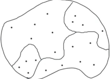
The purpose of a simple random sampling pattern (Figure 2.2) is to ensure that all parts of the project area have an equal chance of being sampled with no operator bias. This condition is important to the assumptions of the underly- ing statistics used in classification. Random sites are selected by dividing the project area into a grid with numbered coordinates. Then coordinate pairs are selected from a random number table and plotted on the project map. Each random point becomes a sample point or the center of a sample area. The size of grid cells is an important consideration that applies to any of these sample patterns and will be discussed later.

Although the simple random pattern leads to a minimum of operator bias, there is a serious drawback to it as a sample pattern. A random pattern over the entire study area is not likely to have a uniform distribution of points, and categories having small areas may be undersampled or missed entirely. Also, some points may prove to be inaccessible.

FIGURE 2.1. The relationship between spectral classes (clusters) and information classes in a hypothetical project. Identification of spectral classes in the field determined that clusters 1 and 2 will merge into a single class, and the same is true for clusters 4 and 5. Because of the similarity in spectral responses for wheat and oats, only one cluster exists for two categories in the map legend. This would necessitate revising the map legend to show the more general term “small grains” rather than trying to include both wheat and oats.

(33)

Stratified Random Pattern

A stratified random sample pattern (Figure 2.3) maintains a necessary randomness and overcomes the chance for an uneven distribution of points among the map categories. This approach assigns a specific number of sample points to each category in proportion to the size or significance of the category with regard to the project objectives. If all categories are of equal significance to the project, then category size alone determines the number of samples in each. To maintain a random pattern, points should be assigned within categories using a grid and random numbers, as in the simple random pattern described previously.

Systematic Pattern

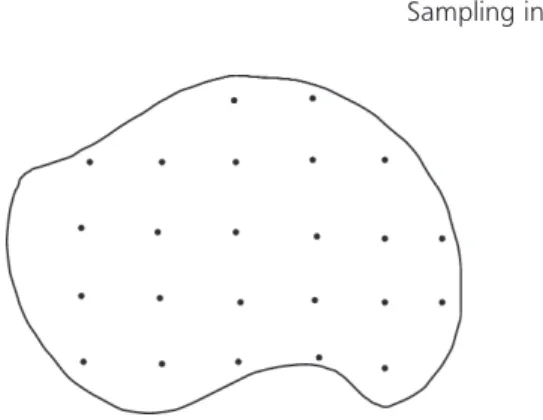
A systematic sampling pattern (Figure 2.4) assigns a sample point to positions at equidistant intervals, for example, all grid intersections. Although the ori-

FIGURE 2.2.Simple random sampling pattern.

FIGURE 2.3.Stratified random sampling pattern.

(34)

entation of the grid may be chosen randomly, because every position is determined by the choice of starting point, randomness is not achieved. This method does not satisfy the assumptions of randomness when using inferential statistics. Another drawback to this method is that such a regular orienta- tion of samples is likely to introduce bias due to some linearity of patterns in the landscape, particularly in regions with a rectilinear land survey system.

Systematic Unaligned Pattern

The systematic unaligned sampling pattern (Figure 2.5) uses a grid, as in the systematic method described above, but assigns the position of each point randomly within the grid cell. In this way a degree of randomness is main- tained within the constraints of the grid cell, but the grid assures that all parts of the project area will be sampled. In order to avoid the tedious operation of devising a pair of random numbers for each cell, it is acceptable to determine

FIGURE 2.4. Systematic sampling pattern.

FIGURE 2.5. Systematic unaligned sampling pattern.

(35)

a random number for each column and for each row of the grid. This approach will result in a random location in each cell.

Using the systematic unaligned sampling pattern assures that sample points will be evenly distributed over the study area and that all classes will be represented. The random position in each may be sufficient to overcome unintended alignments of sample points and landscape features. Whether this is true depends on the size of the cells in the grid. If cells are small relative to landscape alignments, there may still be a problem as described in the systematic sampling pattern. Hence, the crucial issue here is finding the appropriate cell dimension for the grid. Figure 2.5 shows that, by decreasing the size of the cells, a systematic aligned pattern would eventually occur. For example, if there needs to be a large number of samples in order to improve the expected accuracy or the level of confidence, then it would be necessary to have a larger number of smaller cells in the grid. In this situation the element of randomness could be essentially lost.

Clustered Pattern

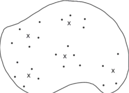
In the clustered sampling approach (Figure 2.6), nodal points are used as cen- ters for clusters of sample points radiating from the center. Any number of nodes can be selected, and any number of satellite points can be tied to them.

Nodal locations can be selected randomly, stratified by category or selected strictly by identification of accessible sites. Furthermore, the satellite points can have random directions and distances from the node even if the node itself was not selected randomly.

From a practical point of view, the clustered sampling approach has some important advantages to a field survey. In terrain with poor access, this

FIGURE 2.6. Clustered sampling pattern.

(36)

method allows the operator to make the most of accessible sites. Another advantage is that field time may be greatly reduced by having fewer sites (nodes), hence less travel time, and multiple satellite sample sites may be vis- ited while at each nodal location. By imposing randomness on the selection of nodes and satellite sites, the assumptions of inferential statistics can still be met. However, the satellite sample sites must be far enough from the nodes to overcome the problem of autocorrelation, thus giving a false statement of map accuracy. Since there is no rule of thumb to follow to determine the distance that a satellite sample site should be from its node, one must be sure that satellite sites are sufficiently far apart to overcome autocorrelation and to make sure that variation within the category is represented. The possibility of autocorrelation is high enough to recommend avoiding the clustered pattern unless other methods are too impractical because of terrain problems.

Purposive or Judgmental Sampling

Purposive sampling is based entirely on the operator’s judgment in purposely, or deliberately, selecting “representative” sample sites. This is defensible if the operator is thoroughly experienced in working with the phenomenon being sampled and is also very familiar with the extent of variation in the study area. The field person’s experience determines where sample sites should be in order to best represent the variation within a category.

The advantage of this approach is that representative sites might just as well be reasonably near roads rather than trekking to a distant site to get the same type of information. However, only a person very familiar with the area would know that the distant site indeed provides the same type of information. This method may be the best option in areas where accessibility to some parts of the study area is a serious problem.

A serious disadvantage is that operator bias is always present, no matter how carefully the work is done. Therefore, statements of accuracy and level of confidence in the final map are statistically invalid, even if the numbers are high, because randomness was not employed. When selecting sample sites purposively, the credibility of the accuracy statement depends entirely on the reliability of the person making the observations. Nevertheless, because of the practicality and ease of site location, this method probably has fairly high usage despite its poor recommendations. If the end user of the project map is also the person most familiar with the area, it may be well to have that person involved in the field when using purposive sampling.

Anyone opting to use the purposive sampling approach should consider taking enough photographs of sample sites to demonstrate that the range of

(37)

variability in each category is represented. When using purposive sampling, care should be taken to use classification programs, such as minimum distance to means, or spectral angles (Sohn & Rebello, 2002), which do not assume randomness of data points.

COMMENTS ON SAMPLING PRACTICALITIES

Some practical considerations must be introduced to the selection of sample sites. One issue is the selection of an appropriate sampling procedure.

Another issue is the acceptance and rejection of certain randomly selected sample sites.

There are two questions regarding rejection of randomly selected sites:

1. What rules should be followed for rejecting samples?

2. If undesirable points are thrown out, is the pattern still random?

Even at the risk of compromising randomness slightly, it is absolutely necessary to reject certain randomly selected points. The most important rule is to reject points lying on boundaries between categories. Every sample site must be wholly within a category. Other criteria for point rejection are more subjec- tive and should be used with caution. For example, as a practical matter, it may be necessary to reject some points because of inaccessibility. However, this rationale can easily be misused and lead to rejection of points that are merely inconvenient. Overuse of this practice would eventually lead to a nonrandom group of sample points. One can imagine carrying this rejection process to an extreme, resulting in a set of “random” samples all located within 200 feet of roads. Any rejected sample point should be replaced by another randomly selected point.

It is important to be clear about sampling procedures when writing the project report. Professional journal articles often omit these details, causing much frustration for project planners looking to the literature for guidance.

Since there are a variety of approaches, each with its advantages and weak- ness, operator integrity requires a frank description of any factors that may contribute to weaknesses in the results. At the same time, the researcher should explain reasons why the methods chosen are well suited for the situation. This openness shows an awareness of the advantages and disadvantages associated with the selected methods and provides a justification based on trade-offs between propriety and practicality, assuming that practicality has not dominated. One must realize, also, that no single correct sampling

(38)

approach applies to all situations. Tests by various researchers have shown that simple random and stratified random patterns both give satisfactory results. However, the stratified random approach requires some advance knowledge of where the strata boundaries are. This is not always possible, but often the probable boundaries can be ascertained with aerial photographs and visits to the field. If unsupervised classification is used as a preliminary step toward supervised classification, the class boundaries are known at the beginning of sampling. This makes it possible to establish a stratified random sample pattern for both the training and the accuracy assessment stages.

NUMBER OF SAMPLES Training Sites

The most important guide for selecting sample sites for training data is to be sure that all the variability within classes is accounted for. In some homogeneous classes this could require only a few sites. More sites will be needed in classes with high variability. A general rule of thumb offered by Jensen (1996) is to select a number of pixels in each class that is at least 10 times the number of bands used in developing training statistics. For example, if 6 bands of TM data are used, then at least 60 training pixels are selected for each class.

This is sufficient to allow valid computations of variance–covariance matrices usually done by classification software. In the discussion below on size of sample sites, it is noted that as sites grow larger than 10 pixels, there may be no new information added. Therefore, it would be better to have six sites of 10 pixels in each class rather than one training site of 60 pixels in each class.

Accuracy Assessment Sites

In spite of efforts by various researchers, there is still no hard and fast rule for determining the number of samples needed for accuracy assessment. How- ever, there are some good guidelines. One suggestion (Fitzpatrick-Lins, 1981) applies the following binomial probability formula to estimate an appropriate number of samples over the entire study area:

N = Z²(p)(q)/E²

where N is number of samples, Z = 2 (the standard normal deviate for a 95%

confidence level), p is expected accuracy, q is 100 – p, and E is allowable error.

For example, if an accuracy of 85% is expected, with an allowable error of 5%

(39)

(95% confidence level), 204 sample sites would be needed to apply this approach. If the allowable error changed to only 2%, the number of samples needed would jump to 1,275. However, this method does not consider the size of the study area, the number of categories, the variation in the areal size of the categories, nor the variability within the categories. It would be very easy to undersample using this method alone unless the confidence level is set to a point that is unrealistic in terms of field time.

A suggestion by Congalton and Green (1999), based on experience with the multinomial distribution, is to use 50 samples minimum in each category.

If the area is larger than 1,000,000 acres, or if there are more than 12 categories, then there should be 75–100 samples per category. This approach samples small areas heavily, while large areas might be undersampled. These suggested sample numbers could be adjusted to accommodate variations in size and within-class variability.

Evaluation of accuracy is an important, though often omitted, part of any project. Although data collection for accuracy assessment may be a job for field personnel, the evaluation is done in the laboratory by means of an error matrix, sometimes called a confusion matrix. This procedure leads to an understanding of accuracy of classification for each category, as well as overall accuracy. Excellent sources for developing a valid evaluation of accuracy include Campbell (1996), Jensen (1996), and Congalton and Green (1999).

SIZE OF SAMPLE SITES

Although the term “sample point” is often used, seldom is it possible to collect data at a single point to represent an area. Point data can be used only when a high degree of generalization is acceptable or when there is no variation in the landscape over an area several pixels in size. For example, point data on a water body is appropriate in projects that are not concerned with variations within a category like water. Be guided by the spectral classes pro- duced by a cluster analysis to assess the uniformity of an information class.

Be aware, however, that a given pixel may change its cluster membership if subsequent cluster analyses have a change in some input parameter, such as maximum number of clusters. Several runs of the cluster analysis program will give an idea of the relative stability of each category. Pixels that consis- tently occur together in the same cluster have good stability and indicate a strongly homogeneous category.

The main things to keep in mind in determining the size of a sample site is

(40)

the variability of the terrain and the ground resolution of the image data, which is usually the same as image pixel dimensions. Remember that the objective is to find a relationship between the single data values in each band of an image pixel and the great amount of information and data in the corresponding ground pixel. Except for applications involving pixel unmixing (subpixel analysis), one will try to generalize a great amount of variation on the ground into a single statement (either qualitative or quantitative) that is representative of an area at least the size of a ground pixel, though usually larger.

In order to associate a particular ground pixel with a specific image pixel, the field person must have precise knowledge of the geographic coordinates of the sample site. Fortunately, satellite global positioning systems have made this task much less difficult than in the past. With selective availability deactivated, location accuracy of approximately 15 meters can be obtained routinely with a hand-held GPS receiver, even without differential correction.

Depending on the configuration of satellites at a given time, accuracy may be even better.

With GPS should a field person try to have sample sites of only one ground pixel in area? This minimal area is not advisable because of errors on the order of 0.5–1.0 pixels, which usually exist in georeferenced images, in addition to errors in ground location. Justice and Townshend (1981) suggest a useful formula for determining area of a sample site:

A = P(1 + 2L)

where A is minimum sample site dimension, P is image pixel dimension, and L is estimated locational accuracy in number of pixels. Suppose, for example, that a project is using TM image data with 30-m pixel dimensions, and one can accurately locate an area on the ground to ±0.5 pixel (15 m). The minimum ground area dimension that should be sampled is 60 m×60 m. Sample sites may be larger than the minimum to allow for a margin of error in ground location and image georeferencing. If operating a GPS without differential correction and without selective availability, a field operator should not estimate a locational accuracy (L) better than 15 m. Keep in mind that the coordinates of a georeferenced image might also have a 15-m error (0.5 pixel) in TM images.

One cannot know the direction of displacement of both the GPS and the image error. They might be additive and create greater total error. Only in areas with a high spatial frequency of variation in surface cover is there a need to strive for minimum sample dimensions. This leads to the consideration of surface homogeneity as a variable in sample site dimensions.

(41)

Homogeneity does not mean there is no variation within a sample, but rather that the variation is uniformly distributed over the area and will produce a unimodal distribution of data. Evaluation of uniformity is very subjec- tive, but Joyce (1978) gave some guidance that is portrayed in Figure 2.7. A more practical and workable guide to homogeneity is the spectral classes pro- duced by cluster analysis. One can assume that each spectral class (cluster) is more or less uniform and is different from other spectral classes. Keep in mind that the cluster maps can vary within the same data set, depending on the parameters set for the clustering process.

Where does this leave us after considering all the variables affecting sample size? How can one best choose a size for sample sites? The practical approach is to identify sample sites based on the size and shape of spectral classes of a cluster map. Sample areas of variable size can be identified within each spectral cluster and located in the field. It is easy to see if a cluster is large enough to locate a sample site safely without danger of location error. As a minimum, sample units should be no smaller than a 3×3 cluster of pixels or a polygon of comparable size for either training sites or accuracy assessment sites. On the other hand, if sample sites are larger than 10–15 pixels, little new information is being added and field time may be wasted. Sample sites containing more pixels add to the amount of field work required at each site.

More information is added by having numerous sample sites of up to 10 pixels each in size.

FIGURE 2.7. The uneven distribution of trees in the figure on the right makes it a poor sample site. The same applies whether considering plants of the same species or an uneven distribution of species in a mixed community. Adapted from Joyce (1978).

(42)

WHERE TO BEGIN MEASUREMENTS

In order to preserve randomness during field work the field person should choose a method for removing bias from the selection of both a starting point and the direction to so in measuring features at specific points along a line, or transect. For example, one might assume that the starting point is the center of a randomly selected sample site. If measurements are to be made along a transect from that point, one should consider a method for selecting a direction for the transect. This might be done by randomly choosing a compass bearing, or by simply flipping a pencil and letting it point in the direction of the transect. This helps avoid choosing a line that is easy to traverse but which may not provide representative data along the way. It would also be valid to select the direction north, or any other direction, and use it for starting a transect at each sample site. This would be sufficient to prevent the field operator from introducing bias in selecting a direction to begin work. The field person may need to select several transects within each sample area in this manner. Note the transect pattern suggested by Joyce (1978) in Figure 2.8.

This approach is valid, and some such approach should be followed consis- tently at each sample area.

If areas, or quadrats, are being used as the basic site for collecting field data, field personnel should have a plan for locating quadrats to be spread over the sample area. For example, one might choose to measure a fixed number of quadrats spaced according to a predetermined plan over each sample area.

The important element of any field work, if randomness is required, is that no bias should be involved in selecting features to measure.

FIGURE 2.8. This suggested transect pattern covers all parts of the sample site and brings the observer back to the point of beginning. The length of the transect will vary according to the size of a given sample site. Adapted from Joyce (1978).

(43)

3

Finding Locations in the Field

Any remote sensing project that requires field measurements, or site-specific observations, must have a means of determining reliable locations for each site. Location in the field before the introduction of a GPS sometimes used surveying techniques such as creating a triangulation net connecting all sample points, but most often relied on identifying landmarks on the ground that could also be seen on the image (e.g., bridges, intersections of roads or streams). The field person had to take samples adjacent to, or a measured distance from, the landmark. This restriction greatly hampered taking samples in remote areas with few landmarks unless the area to be sampled was large and fairly homogeneous, allowing for large errors in location. One simply accepted the possibility that locational accuracy would be weak.

In urban areas, or well-developed agricultural areas, the locational problem was less restrictive due to the abundance of easily identified landmarks.

Using those early techniques for location in the field often required that a large number of contiguous pixels be used for each site, whether used for training, field sampling, or verification. Field personnel still find it useful to 26

(44)

know how to follow a bearing with a compass and to make measurements by pacing, taping, or using devices such as the hip chain, which uses an unwind- ing string to record the distance a person walks. However, today’s GPS technology is absolutely vital to finding locations in the field and must not be ignored. Every researcher who plans to do field work in remote sensing must have access to a GPS receiver and learn to use it proficiently.

The advent of GPS technology in the 1980s and the completion of the satellite array in 1995 have greatly changed the approach to location-finding in the field. With selective availability deactivated since May 2000, location accuracy of 15 m or better is obtained routinely 95% of the time with a handheld GPS receiver and without using differential correction. Depending on the geo- metric configuration of satellites at a given time, estimated accuracy is often much better than 15 m. An inexpensive GPS receiver can enable remote sensing field workers to navigate with confidence to a point on the ground with known coordinates derived from a map or georeferenced image. Or it can help them determine such coordinates for sample points selected in the field.

Both of these functions have important applications in remote sensing projects and will be discussed in detail later in this chapter. What will not be covered in depth is the actual operations of the GPS. This is because the purpose of the chapter is to acquaint field personnel with field procedures using GPS.

For greater detail on system operation, recommended readings are Geomatics Canada (1995), French (1999), VanSickle (2001), and Hurn (1989).

OVERVIEW OF LOCATION-FINDING USING GPS

The U.S. Department of Defense initiated the system, called NAVSTAR GPS, which provides the best means available for navigation and position location.

The system is an array of 24 orbiting satellites that emit radio signals, including three spares for backup. All the satellites are in 12-hour orbits at just above 20,200 kilometers (km; 12,500 statute miles) above the surface of the earth, and are arrayed so that at least four are available for use at any location between about 80° north and south latitude. Four satellites are the minimum needed to obtain reliable positions and elevations. It is desirable to have a receiver that will track at least eight satellites (some will track 12) so that the best four can automatically be selected for position computation. If one of the four satellites deemed optimal for location computation should move out of view over the horizon, another is already on track to fill in as necessary.

When a GPS receiver is turned on, it first downloads a current almanac of

(45)

all the satellites, whether in view or not. The satellites that are in view may then be shown on the GPS receiver screen. Usually the display is on an azimuthal grid with the center at the user’s location. Also, there may be a display showing signal strength either as a bar graph or as a number next to the satellite plotted position. Each satellite has a unique signal code that identifies it to the receiver on the ground. If a receiver has not been used for several months, or is more than 300 miles from its last position, it will need to initial- ize and may request operator input on the approximate present location.

One may obtain updated satellite almanac information on the positions of satellites, including satellite visibility and geometry before going into the field. Almanacs and other information on the satellites in the NAVSTAR con- stellation can be obtained on the U.S. Naval Observatory website, http://

tycho.usno.navy.mil/gps.html. Select “GPS Interactive Satellite Visibility,” and input latitude and longitude of the field area of interest and the expected date of the field trip. The result will be a list of optimal satellites at that time and place. One can then try some alternate dates and hours to compare with the first results. With this almanac information, the user can create a chart for a given location showing the days and hours of optimal satellite coverage. Fig- ure 3.1 is an example of such a chart. A blank azimuthal chart is provided in Appendix 2.

Two means of taking position observations may be utilized by field workers in remote sensing single-point location and differential location. Differen- tial location requires that data be collected from two locations simultaneously.

Although differential location can achieve submeter accuracy, its use is limited in remote sensing projects if navigation to a known point is needed. However, when points are selected and their positions recorded in the field, differential location correction may be warranted if accuracy needs require it. For most purposes, single-point location will provide adequate accuracy unless the signal degradation called Selective Availability is turned on again sometime in the future.

Single-Point Location

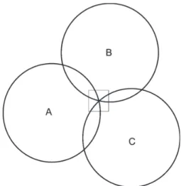
Location of a point operates on the principle of intersecting circles marking a point (Figure 3.2). The circles represent all equidistant points between each satellite and the GPS receiver on the ground. The intersection of the circles determines the actual location of the receiver. The diagram in Figure 3.2 is a two-dimensional representation that does not show the effects of tiny, but significant, clock error in the receiver instrument. In practice, a fourth satellite

(46)

signal is needed to compensate for small time discrepancies in the receiver instrument’s clock. Hence, a minimum of four satellites is required to determine a location.

Dif ferential Location Measurements

Greater location accuracy requires a stationary GPS station that records data continuously while a roving receiver takes data at selected points in the field.

Fixed stations are operating continuously in many places now, and may be located as much as 300 miles from the roving receiver. Check with a local sur- veyor’s office for information on operational base stations in the area of interest. When the field personnel return to home base they can download into a FIGURE 3.1. Radial lines represent azimuths and concentric rings represent ele- vation angles. The outer ring represents a mask that screens out any satellites less than 15° above the horizon. The paths of five satellites, identified by number, are plotted over a 2-hour period. Not all GPS equipment has the capability for making these plots, but with information on the U.S. Naval Observatory website such plots can be made by hand. Adapted from Geomatics Canada (1995). Used with permission.

(47)

computer both the roving data and the fixed station data for the time period they were in the field. Software obtained with certain receivers will make the appropriate signal matches and compute differential corrections for all locations obtained by the roving receiver. An explanation of the details of this procedure would be specific to various manufacturers’ software and is beyond the scope of this book.

Sources of System Error

Inherent in the NAVSTAR GPS system are errors that include orbital errors, satellite clock errors, ionospheric path errors, receiver clock errors, and receiver noise related to instrument design. These sources of error are beyond the control of the field person during a field survey, but the operator can control for other possible error sources.

FIGURE 3.2. This two-dimensional version of the geometry on which position computations are made shows that signals from three satellites define a point location. The distance from satellite A applies to any point on circle A. The same applies to circles B and C. The intersection of the three circles, shown within the square, is the only correct location. The NAVSTAR system operates in three dimensions, and location is computed on the intersections of spheres rather than circles. The intersection of three spheres forms two widely separated points, but one of them is easily identified as an incorrect solution. Adapte