The Industrial and Systems Engineering Handbook is the latest addition to the collection of industrial and systems engineering knowledge. There is a growing need for a handbook on the ever-expanding field of industrial and systems engineering.
GENERAL INTRODUCTIONS
FUNDAMENTALS OF INDUSTRIAL ENGINEERING
FUNDAMENTALS OF SYSTEMS ENGINEERING
MANUFACTURING AND PRODUCTION SYSTEMS
NEW TECHNOLOGIES
GENERAL APPLICATIONS
FUNDAMENTALS OF
INDUSTRIAL ENGINEERING
Human Factors in Industrial and Systems Engineering
Human Factors are important to industrial and systems engineering because of the prevalence of humans in industrial systems. However, the prevalence of poor design suggests that Human Factors acumen is not as common as one might think.
Elements of Human Factors
- Cognition
- Behavior
- Performance
- Reliability
- The Benefits of Human Factors
There are many benefits to considering each of these four elements of Human Factors in system design. Consideration of human factors also leads to cost reductions in system design, development and production.
A Human Factors Conceptual Model
- Long-Term Memory
- Types of Long-Term Memory
- Implications for Design
- Case: Power-Plant Control
- Working Memory
- Implications for Design
- Case: Cockpit Checklists
- Sensation
- Implications for Design
- Case: Industrial Dashboards
- Perception
- Implications for Design
- Case: In-Vehicle Navigation Systems
- Attention and Mental Workload
- Implications for Design
- Case: Warnings
- Situation Awareness
- Implications for Design
- Case: Air-Traffic Systems
- Decision-Making
- Diagnosis
- Choice
- Decision-Making Heuristics
- Implications for Design
- Case: Accident Investigation
Expectations can be described as the beginning of the schema for the object that is expected. Workers can be trained to focus on the most diagnostic resources in each decision area.
Cognitive Consequences of Design
- Learning
- Implications for Design
- Error
- Implications for Design
Because skill-based behavior requires little attention, the response is often completed before the error is noticed. For example, when anticipating a skill-based behavior, prominent feedback should be designed into the display interface to ensure that employees are aware when a mistake is made.
Summary
Marble, J.L., Medema, H.D., and Hill, S.G., Examining decision-making strategies based on information acquisition and information search time, Proceedings of the Human Factors and Ergonomics Society 46th Annual Meeting, Human Factors and Ergonomics Society, Santa Monica, CA, 2002. Roth, E.M., Gualtieri, J.W., Elm, W.C., and Potter, S.S., Scenario Development for Decision Support System Evaluation, Proceedings of the Human Factors and Ergonomics Society 46th Annual Meeting, Human Factors and Ergonomics Society, Santa Monica, CA, 2002.
Introduction
Immediately, the pressure in the primary system (the core part of the plant) began to increase. The purpose of this chapter is to focus on recent issues in the study of HF.
History of Human Factors
Instead, the operators estimated the water level in the core from the pressure level, and since it was high, they assumed the core was properly covered with coolant. In the early era of HF research, improving productivity was the primary focus, but as technology has advanced, especially computer technology, the usability of computer tools, machines, and software has moved to the forefront of research topics.
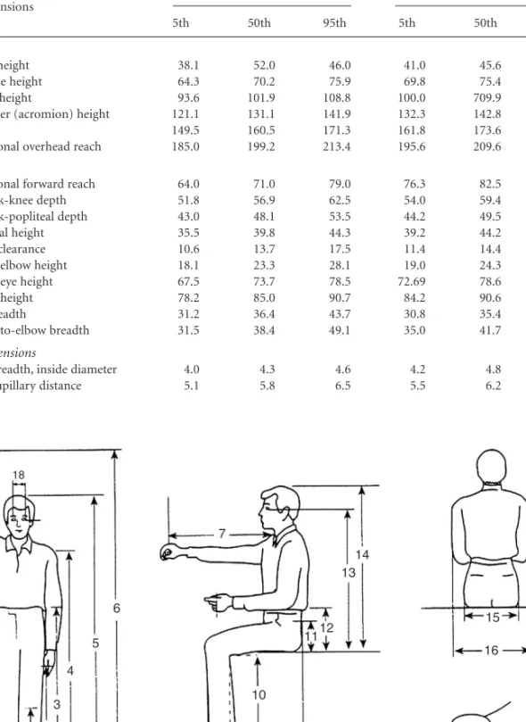
Anthropometry
1945 to 1960 ● The HF profession was born; HF study in the United States was essentially concentrated in the military-industrial complex. At the end of the war in 1945, engineering psychology laboratories were established in the United States and Britain.

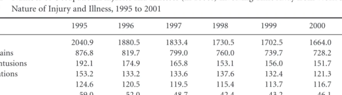
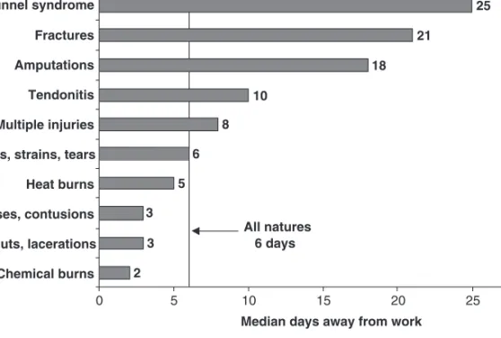
Work-Related Injuries: Musculoskeletal Disorders
There are three design principles when designing for most individuals: design for extremes, design for the average, and design for adjustability (Niebel and Freivalds, 2003). Design for adjustability is typically used for equipment or facilities that can be adjusted to fit a wide range of individuals.
Epidemiological Research Methods
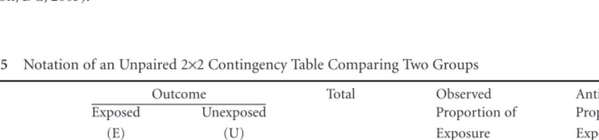
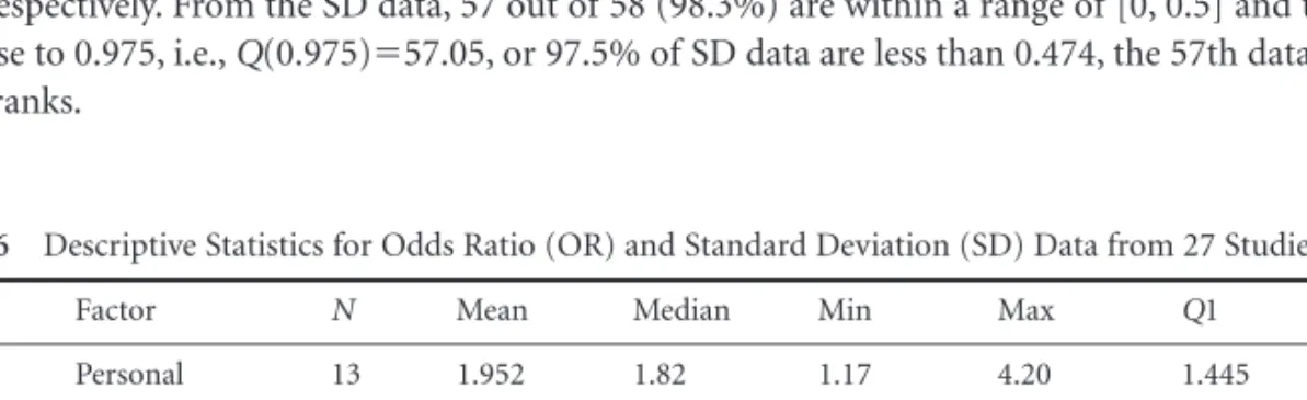
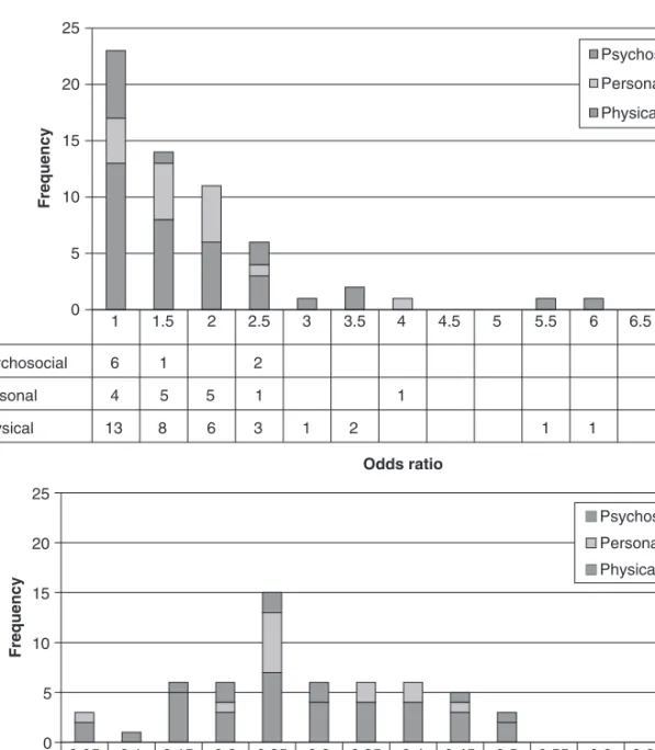
In a case-control study, the odds of exposure in each group indicate a proportion of the probability of an outcome (p) to its complementary probability (1⫺p), as formulated in equations (2.1) and (2.2). the odds of exposure of the case group and the odds of exposure of the control group, respectively. Based on the literature survey, risk factors for SST were grouped into three main categories: (1) personal factors, (2) psychosocial, and (3) physical factors.
CA/U ⫻ X CO/EXCA/E/XCA/U
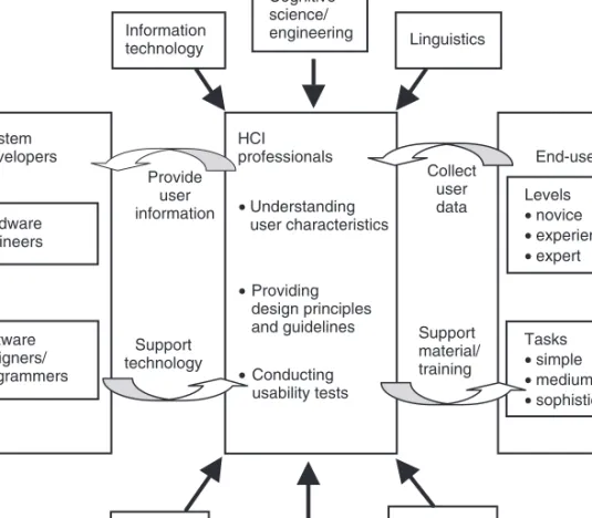
Human–Computer Interaction
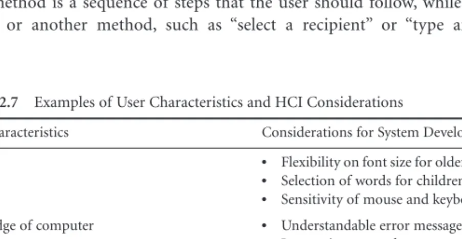
- Understanding User Characteristics
- Providing Design Principles and Guidelines
- Conducting Usability Tests
The HCI professionals also provide the user with more user-friendly support materials with the help of system developers. The goal of the HF specialist is to narrow this gap by understanding and paying attention to user needs rather than what the system developers want to make.
Summary
Low-fidelity methods commonly used early in the design process include index cards, paper stickers, paper-and-pen drawings, and storyboards. High-fidelity methods include fully interactive displays with the look and feel of the final software (Wickens et al., 2004).
Exercises
Hagberg, M., Morgenstern, H., and Kelsh, M., Impact of occupations and work tasks on the incidence of carpal tunnel syndrome, Scand. Miller, R.F., Rapids, C., Lohman, W.H., Maldonado, G., and Mandel, J.S., An epidemiological study of carpal tunnel syndrome and hand-arm vibration syndrome in relation to vibration exposure, J.
Introduction
On the other hand, practitioners of EPC criticize SPC methods for excluding the opportunities for reducing the variability in the process output. Recently, an integration of EPC and SPC methods has emerged in semiconductor manufacturing and has led to a tremendous improvement in industrial efficiency (Sachs et al., 1995).
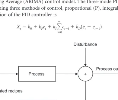
Two Process-Control Approaches
- Engineering Process Control
- Statistical Process Control
- Common-Cause Variations
- Special-Cause Variations
On the other hand, once the process output deviates from the target, corrective action is initiated regardless of the source and type of disturbance. With few exceptions, the mean of the process is constant except for occasional sudden changes, i.e. ηtηµt.
Integration of Engineering Process Control/Statistical Process Control — Run-to-Run Control
- Diagnosis Module
- Gradual Module
- Rapid Module
For example, when the process can be described by an ARIMA model, the MMSE control has a form identical to that of the MMSE predictor (Box et al., 1994). Mandel (1969) suggests monitoring the prediction errors; and Zhang (1984) suggest cause-selective control charts to determine which of the inputs or outputs are responsible for the out-of-control situation.
A Run-to-Run Example — Chemical–Mechanical Planarization
For illustration, we consider the control output wafer thickness using polishing pad rotation speeds. Note that although the original EWMA controller is designed to reduce input dielectric variations, the severity of the pad degradation is also weakened (the operation has been reduced to a step change).
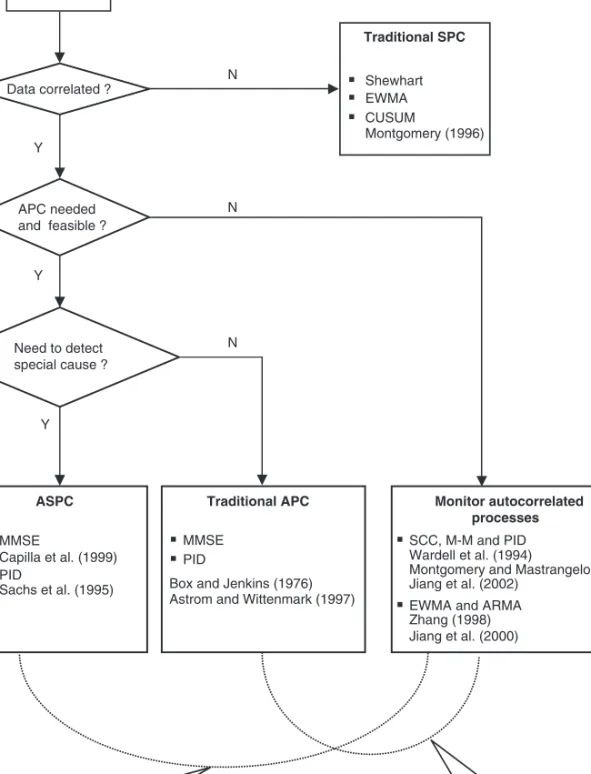
Monitoring Autocorrelated and Engineering Process Control Processes
- Modifications of Traditional Methods
- Forecast-Based Monitoring Methods
- Generalized Likelihood Ratio Test-Based Multivariate Methods
- Batch Means Monitoring Methods
- Monitoring Integrated Engineering Process Control/Statistical Process Control Systems
- Design of Statistical Process Control Methods: Efficiency vs. Robustness Although EPC and SPC techniques share the same objective of reducing process variations and many
They show that the SCC chart is a special case of the WBM method and that monitoring series averages can be more effective at detecting small mean process shifts than forecast-based charts. Similarly, the residual diagram is equivalent to the associated monitoring component of the EPC/SPC system.
Concluding Remarks
Sachs, E., Hu, A. and Ingolfsson, A., Process control after startup: combining SPC and feedback control, IEEE Trans. Wardell, D.G., Moskowitz, H. and Plante, R.D., Length distributions of special cause control charts for correlated observations, Technometrics.
Introduction
- Key Milestones
Each person involved in the project may need a schedule with all the activities in which they are involved. Key milestones should be defined for all major phases of the project before starting.

Estimating the Duration of Project Activities
- Stochastic Approach
- Deterministic Approach
- Modular Technique
- Benchmark Job Technique
- Parametric Technique
Collect data on past performance time of the activity for different values of the independent variables. In the first step, a simple regression equation is developed with the independent variable that is the best predictor of the dependent variable (ie the one that produces the highest value of R2).

Precedence Relations among Activities
Other types of connections are examined in Section 4.8, and the effect of uncertainty on preference ratios is discussed in Section 4.10. Three models used to analyze priority relationships and their schedule effects are the Gantt chart, CPM, and PERT.
Gantt Chart
As shown in Figure 4.13, which shows the Gantt chart for the microcomputer development project, a separate column can be added for this purpose. In Figure 4.13, a bold border is used to identify a critical activity, and a shaded area indicates the approximate completion status at the August review.
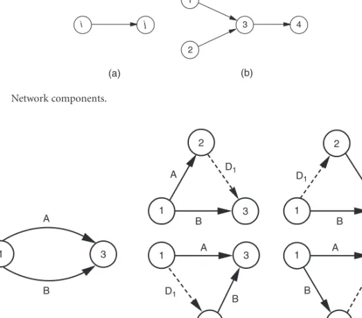
Activity-on-Arrow Network Approach for Critical Path Method Analysis
- Calculating Event Times and Critical Path
- Calculating Activity Start and Finish Times
- Calculating Slacks
This implies that the three arrows representing these activities can end at the same node (event) - the tail of F. Thus, applying equation (4.4), the end time of event 2 is the minimum between the late times dictated by the two sequences . ; this is,.
Activity-on-Node Network Approach for Critical Path Method Analysis
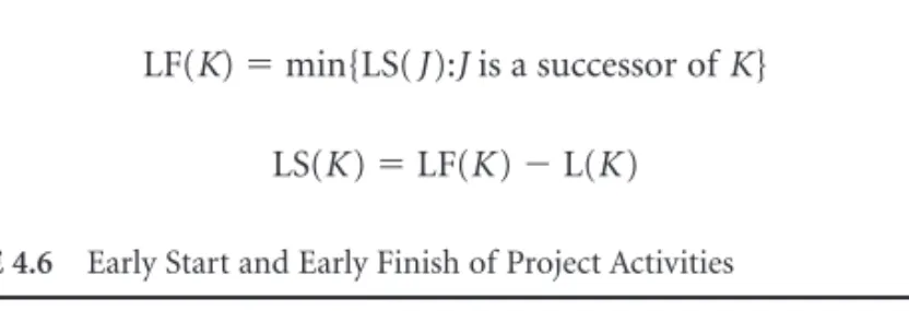
- Calculating Early-Start and Early-Finish Times of Activities
- Calculating Late Start and Finish Times of Activities
Thus, the EC time of an activity is equal to the maximum early completion (EF) time of all activities immediately preceding it. The ES time of the initial activity is assumed to be zero, as is its EF.
Precedence Diagramming with Lead–Lag Relationships
Depending on the nature of the tasks involved, an activity does not have to wait until its predecessor is finished before it can start. Figure 4.29 shows the Gantt chart for the example incorporating the lead-lag constraints. Since the original duration of C is 10 days, the duration of C1 is calculated to be 10 2 8 days. Figure 4.31 shows a conventional AON network drawn for the three activities after they are divided into separate parts.

Linear Programming Approach for Critical Path Method Analysis
The duration of C2 is 2 days because there is an FF2 relationship between activity A and activity C. It should also be noted that the different segments of each activity are performed consecutively.
Aggregating Activities in the Network
- Hammock Activities
- Milestones
A higher level of aggregation is also possible by introducing milestones to mark the completion of significant activities. In the simplest case, a milestone can mark the completion of a single activity, as event 2 in our example marks the completion of activity A.
Dealing with Uncertainty
- Simulation Approach
- Program Evaluation and Review Technique and Extensions
Thus, a simple PERT estimate (based on the critical sequence A–B–E) shows that the probability of completing the project in 17 days is 29%. Based on a simple PERT analysis, the probability of completing the project in 22 weeks is 0.5.

Critique of Program Evaluation and Review Technique and Critical Path Method Assumptions
Of the two, the Chebyshev estimate is probably more reliable since there are few activities on the critical path. The contractor who is on the critical path generally has more leverage in obtaining additional funds from these contracts because he or she has a large say in determining the duration of the project.
Critical Chain Process
On the other hand, some contractors deem it desirable to be less “visible” and therefore adjust their time estimates and activity descriptions so that they do not end up on the critical path. Management must ensure that those in charge of monitoring and controlling the performance of activities have a working knowledge of the statistical characteristics of PERT and the general nature of critical path planning.
Scheduling Conflicts
Neumann, K., Schwindt, C., and Zimmermann, J., Time Windowed and Resource Constrained Project Scheduling: Time and Constrained Project Scheduling with Regular and Irregular Objective Functions, Lecture Notes in Economics and Mathematical Systems, Vol. Fisher, D.L., Saisi, D., and Goldstein, W.M., Stochastic PERT networks: OP diagrams, critical paths, and project completion time, Comp.
Cost Concepts and Definitions
These are costs that represent the normal or expected cost of a unit of an operation's output. These are costs that vary directly according to the level of business or the amount of output.
Cash Flow Analysis
- Time Value of Money Calculations
- Effects of Inflation
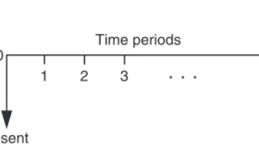
The size of the cash flow in the gradient series at the end of period t is calculated as. The cash flow starts with a positive base amount, A1, at the end of period 1. Figure 5.8 shows a decreasing geometric series.
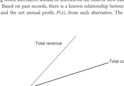
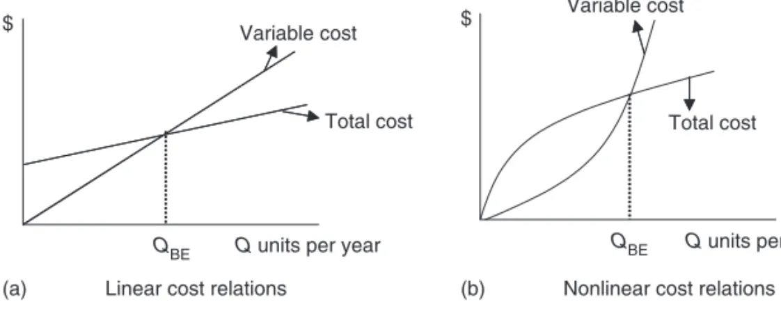
Break-Even Analysis
- Profit Ratio Analysis
In addition to the break-even points, other value measures or criterion measures can be derived from the charts. Profit margin is defined as the ratio of the profit area to the sum of the profit and loss areas in a break-even chart, i.e.
Amortization of Capitals
It is desirable to carry out a detailed analysis of the loan schedule. Table 5.2 provides a partial overview of the loan repayment schedule. Keep in mind that very little equity is built up during the first three years of the loan schedule.
Manufacturing Cost Estimation
The percentage of interest charge in the monthly payments starts at 77.55% for the first month and drops to 0.83% for the last month. In comparison, the percentage of interest in the total payment also starts at 77.55% for the first month and slowly decreases to 48.30% by the time the last payment is made at time 180. Table 5.2 and Figure 5.18 show that an increasing proportion of the monthly payment goes into the principal payment as time goes on.
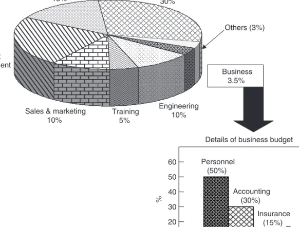
Budgeting and Capital Allocation
The level of accuracy associated with detailed estimates normally ranges from −5 to ⫹5% of actual costs. This translates into an ROI of 83.92%. Figure 5.22 presents histograms of investments and returns for the four projects.
Cost Monitoring
Project Balance Technique
Cost and Schedule Control Systems Criteria
In the conventional approach, it is possible to misrepresent the actual content (or value) of the work done. The work rate analysis technique presented in section 35.3 may be helpful in overcoming the shortcomings of the conventional approach.

Sources of Capital
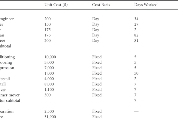
Activity-Based Costing
The specific ABC cost components shown in the table can be broken down further if necessary. Based on this analysis, it can be seen that product line A is the most profitable.
Cost, Time, and Productivity Formulae
The learning effect limit indicates the number of times a task is performed at which no further improvement is achieved. -Sinking Fund Factor Series • Uniform Series Compound Quantity Factor • Arithmetic Gradient Series Factor • Tent Cash Flow Equation • Geometric Gradient Series Factor.
Introduction
Some of the software tools used for engineering economic evaluations are presented in Appendix A, and a bibliography of some of the excellent textbooks on engineering economic analysis techniques is in References.
Cost Estimation Techniques
- Time-Series Techniques
- Correlation and Regression Analysis
- Exponential Smoothing
- Subjective Techniques
- The Delphi Method
- Technological Forecasting
- Cost Engineering Techniques
- Unit Technique
- Ratio Technique
- Learning Curves
An interquartile range of the opinions is calculated and presented to the participants at the beginning of the second round. It recognizes that cost varies as a function of the change in capacity of size.
Interest Rates in Economic Analysis
- Nominal and Effective Interest Rates
- Fixed and Variable Interest Rates
- Rule of 72 and Rule of 100
The compound interest rate (or interest rate for short) is used in economic analysis to calculate the time value of money. If interest rate differences are not large, cash flow calculations usually ignore the effect of interest rate changes.
Cash-Flow Analysis
- Compound Amount Factor
- Present Worth Factor
- Uniform-Series Present Worth Factor
- Capitalized Cost Formula
- Uniform-Series Capital Recovery Factor
- Uniform-Series Sinking Fund Factor
- Uniform-Series Compound Amount Factor
- Arithmetic Gradient Series Factor
- The Tent Cash-Flow Equation
- Geometric Gradient Series Factor
The closed form of the PW of an arithmetic gradient series with a zero base amount is. However, the formula for calculating the PW of the descending geometric series of cash flows is (Badiru, 1996).

Economic Methods of Comparing Alternatives
- Present Worth Analysis
- Capitalized Cost
- Discounted Payback Period Analysis
- Annual Worth Analysis
- Permanent Investments
- Internal Rate of Return Analysis
- External Rate of Return Analysis
- Benefit/Cost Ratio Analysis
- Incremental Analysis
Column C: PW at the given interest rate for the respective net cash flow in column A. P⫽the present value of all cash flows at MARR F⫽the future value of all cash flows at MARR i′⫽the unknown ERR.
Replacement or Retention Analysis
- Economic Service Life
- Replacement Analysis
- When Defender Marginal Costs can be Computed and are Increasing
- When Defender Marginal Costs can be Computed but are not Increasing
- When Defender Marginal Costs cannot be Computed
Plot costs against both the minimum EUAC of the challenger and the marginal cost of the defender. Hold the defender for at least the number of years its marginal cost is less than the minimum EUAC of the challenger.
Depreciation and Depletion Methods
- Depreciation Methods There are five principal depreciation methods
- Straight-Line Method
- Declining Balance Method
- Sum-Of-Years’-Digits Method
- Modified Accelerated Cost Recovery System Method
- Depletion Methods
- Cost Depletion
- Percentage Depletion
Depreciation: The annual depreciation amount, Dt, is the declining value of the asset to the owner. Salvage value: Estimated trade-in or MV at the end of the asset's useful life.
Effects of Inflation on Economic Analysis
- Foreign Exchange Rates
If the series is expressed in today's dollars, then the discounted cash flow uses a real interest rate. However, the compounding rate is applied if the series is denominated in future dollars.
After-Tax Economic Analysis
- After-Tax Economic Analysis
ATCF estimates are used to calculate PW, AW or FW at the after-tax MARR. Column E: After-tax cash flow for direct use in economic valuation techniques or after-tax analyses.
Decision-Making Under Risk, Sensitivity, and Uncertainty
- Sources of Uncertainty in Project Cash Flows
- Non-Probabilistic Models
- Probabilistic Models
When one of the parameters of an evaluation technique, such as P, F, A, I, or n for a single project, is not known or cannot be estimated with certainty, a break-even technique can be used using the equivalent ratio for the Set PW , AW, ROR or B/C equal to 0 to determine the break-even point for the unknown parameter. The results of this approach can be compared to decision making when parameter estimates are made with certainty.
Appendix A: Software Tools for Economic Analysis
Select the parameters in each alternative to be treated as random variables and estimate values for other particular parameters. Calculates the depreciation schedule using the DB method with a shift to SLN in the year where straight-line has a larger depreciation amount.
The Other Software Tool
- Introduction
- Basic Concepts of Work Sampling
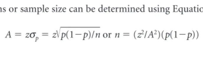
- Accuracy
- Confidence Interval
- Sample Size
- Random Observation Times
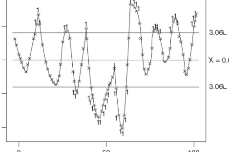
- Control Charts
- Plan of a Typical Work Sampling Study
- Applications of Work Sampling
- Machine Utilization
- Allowances for Personal and Unavoidable Delays
- Summarizing the Sampling Data The ABC study is summarized in Table 7.4
- Determining Work Standards
- Computerized Work Sampling
- Conclusion
Work samples are best suited for determining (1) machine utilization, (2) taking into account unavoidable delays, and (3) work standards for direct and indirect work. Waddell, H.L., Work sampling – a new tool to save costs, increase productivity, make decisions, Factory Manage.
FUNDAMENTALS OF SYSTEMS ENGINEERING
Summary
Introduction
Each of these fields makes a particularly positive contribution to the growth of industrial and systems engineering. Computers are helpful in CAD/CAM, which is an important area of industrial and systems engineering.