The presentation of a technique for solving these systems of equations is one of the contributions of this book. Therefore, executable program elements are included on the CD that can be used directly, without compilation, to solve some, but not all, of the problems in this book.
REVIEW OF FUNDAMENTALS
THE FUNDAMENTAL PRINCIPLES .1. THE BASIC EQUATIONS
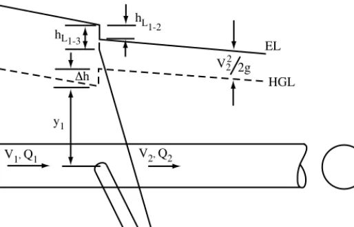
- ENERGY AND HYDRAULIC GRADE LINES
The last two terms, however, are extremely important in the study of pipeline hydraulics. Fluid power, sometimes denoted P, is the product of the energy gain or loss per unit weight hm and the weight rate of flow Qγ, or P = Qγhm.
HEAD LOSS FORMULAS
- PIPE FRICTION
- DARCY-WEISBACH EQUATION
- EMPIRICAL EQUATIONS
- EXPONENTIAL FORMULA
- LOCAL AND MINOR LOSSES
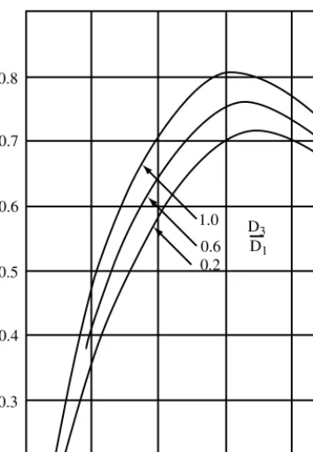
The Hazen-Williams and Manning equations can be solved for hf and put in the form of the exponential formula. To find K and n for the Darcy-Weisbach equation, we note that f can be approximated over a limited region on the Moody diagram by an equation of the form
PUMP THEORY AND CHARACTERISTICS
A change in the shape of a curve normally means that the flow pattern within the pump has also changed. For the operating discharge, read NPSH from the pump curve, after which zi can be calculated.
STEADY FLOW ANALYSES
- SERIES PIPE FLOW
- THREE RESERVOIR PROBLEM
If the flow is assumed to be in the fully coarse flow region of the Moody diagram, Fig. In this case, hp is the total discharge pressure developed in the three stages of one of the two pumps.
PROBLEMS
Use the K and n values that were found in Example Problem 2.1 from the Darcy- Weisbach, Hazen-Williams and Manning equations to compute the head losses associated
2 2 The pump below delivers 8 ft3/s of water. a) Draw a diagram of the system and locate the EL and HGL at sections 1 and 2 in the diagram.
To obtain more electrical energy during the day when there is a shortage and use it during the late night when there is a surplus, a power company plans to pump water from
Write a program for a computer or calculator for determining the unknown diameter of a pipe (Category 3), including local losses
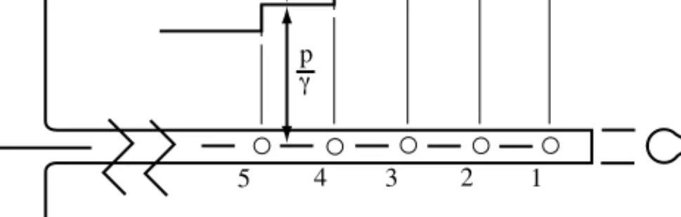
MANIFOLD FLOW
- INTRODUCTION
- ANALYSIS OF MANIFOLD FLOW
- NO FRICTION
- BARREL FRICTION ONLY
- BARREL FRICTION WITH JUNCTION LOSSES
- A HYDRAULIC DESIGN PROCEDURE
- PROBLEMS
- In the manifold shown below, neglect all losses except pipe friction in the barrel, and assume f = 0.02 is a reasonable estimate for the Darcy friction factor in the barrel
- Certain assumptions are made in the analysis of a major submarine diffuser manifold for the disposal of wastewater. Indicate which of the following assumptions is both correct
- Devise a computational scheme to determine the head loss across a port in the main line of a manifold. Implement the scheme in the manifold program MANIFOLD on the
- Trickle irrigation of a field may involve a hierarchy of manifolds; that is, a delivery main can serve as the supply to several manifolds, and each manifold will in turn serve a
All parts of the power line slope down in the direction of flow in the main and lateral part, due to. At the high end of the spectrum we note that the main flow in
PIPE NETWORK ANALYSIS
INTRODUCTION
- DEFINING AN APPROPRIATE PIPE SYSTEM
- BASIC RELATIONS BETWEEN NETWORK ELEMENTS
For a loop network, the number of loops (around which independent energy equations can be written) is given by The number of pseudo-loops numbered as part of NL is equal to the number of supply sources minus one.
EQUATION SYSTEMS FOR STEADY FLOW IN NETWORKS Three different systems of equations can be developed for the solution of network
- SYSTEM OF Q - E Q U A T I O N S
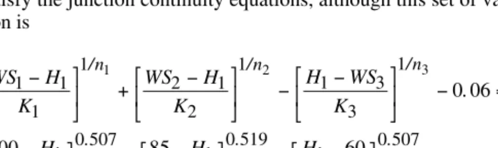
The coefficients K and n for the exponential formula are given in the table for each of the three pipes in this branched system. In this network, two independent continuity equations are available, and consequently the head must be specified at one of the junctions. To obtain these equations, we replace the discharge in each pipe of the network by an initial letter.
The junction continuity equations are satisfied by the initial discharges Qoi and are not part of the system of equations. The next step is to find an initial estimate for the discharge in each pipe that will satisfy all the junction continuity equations. By writing the ∆Q equations we must also give values for Qoi that satisfy all the intersection continuity equations.
PRESSURE REDUCTION AND BACK PRESSURE VALVES A pressure-reducing valve (PRV) is designed to maintain a constant pressure at its
- Q-EQUATIONS FOR NETWORKS WITH PRV'S/BPV'S
- H -EQUATIONS FOR NETWORKS WITH PRV'S/BPV'S
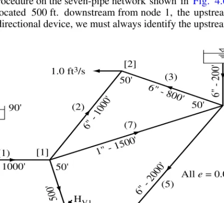
The second loop must extend from the artificial reservoir created by the PRV to one of the other supply sources (or another artificial reservoir, if two or more PRVs exist in the network). When writing the head loss in pipe 6, only that section of the pipe downstream of the PRV is used. We will denote this variable by Hvi, where i is the number of the device.
To illustrate the writing of the ∆Q-equations, let's look again at the PRV network shown in the figure. In this network, the three PRVs cause the pressures at nodes 4 and 6 to be independent of the pressures in the rest of the network. If this calculated NP exceeds the number of pipes in the network, then PRVs isolate part of the network.
SOLVING THE NETWORK EQUATIONS
- NEWTON METHOD FOR LARGE SYSTEMS OF EQUATIONS In Sections 4.2 and 4.3 we explored the writing of systems of algebraic equations to de-
- SOLVING THE THREE EQUATION SYSTEMS VIA NEWTON The Newton method will now be applied in turn to the solution of the Q-equations, the
- COMPUTER SOLUTIONS TO NETWORKS
- INCLUDING PRESSURE REDUCING VALVES
The first part of the main program is currently written specifically to solve the Q equations for the three-reservoir problem. In the Q-equations the Jacobian elements will be either ∂Fi/∂Qj = ±1 or zero in row i for a row of the intersection continuity equation. There are also local loss devices in tubes 7, 8, and 3, the first two of which have a loss coefficient of 10, and the third has a loss coefficient of 2. Roman numeral loop notation will be used in Example Problem 4.6. ).
Next let us consider the formulation and solution of the H equations for the network in Example Problem 4.6. In the next two sections, similar programs will be developed for solving H equations and ∆Q equations. A line giving (a) the number of pipes, (b) the number of nodes, (c) the number of tanks supplying the network, (d) the number of pumps, and (e) the options you want to change from the default values. The default options and how to change them will be described later.).
For each reservoir, (a) the pipe number connecting this reservoir to the network and (b) the water surface elevation of the reservoir are listed. From this information develop the system of Q equations, i.e. the connection continuity equations and the energy equations around pseudo and real loops in the network.
PROBLEMS
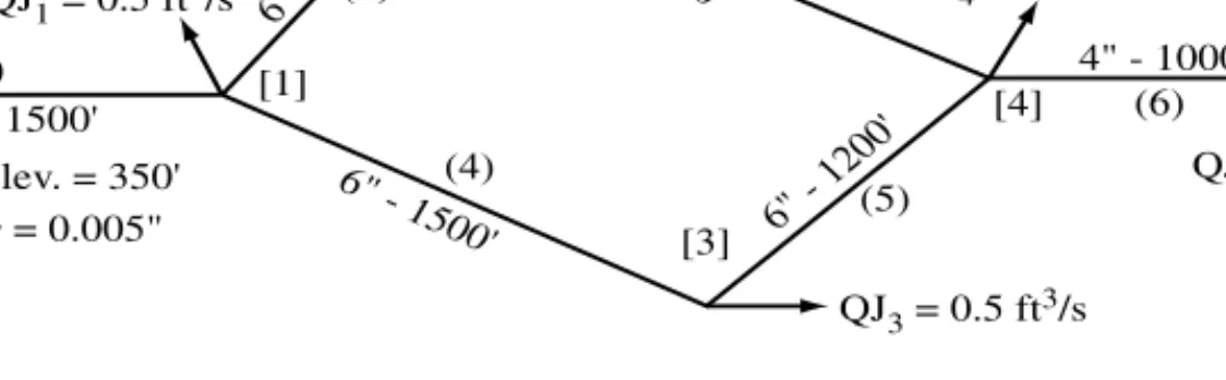
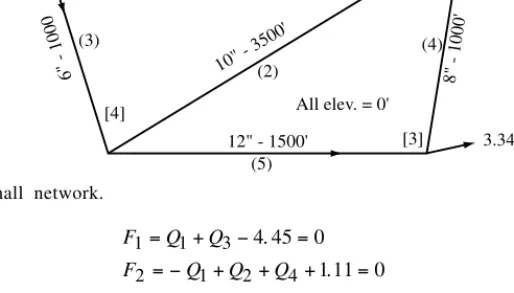
In this diagram, the first number along each line is the diameter of the pipe in inches, and the second number is the length of the pipe in feet. Do the following: (a) calculate the values of K and n in hf = KQn for tube 1 based on the Darcy-Weisbach equation, and (b) write the system of Q-equations for this network. Use subscripts on K, n, and Q corresponding to tube number.). The values of K and n for pipes in this network are given in the table below.
Prepare the input data for, and obtain the solution from, NETWK for the network described in Problem 4.6
Write the system of H-equations for the two networks in Problem 4.1
2 0 For the network shown: (a) write the Q-equations; (b) write the H-equations;. c) write down the ∆Q-equations; and (d) solve the system of ∆Q-equations.
For the two networks in Problem 4.1, solve the Q-equation system using the New- ton method
For the two networks in Problem 4.1, solve the H-equation system using the New- ton method
For the two networks in problem 4.1, solve the system of equations Q using Newton's method. Use the Hazen-Williams equation to analyze this network; all pipes are cast iron. Use the Hazen-Williams equation to analyze this network that is diagrammed on the next page; all pipes are cast iron.
Modify SOLHEQS so it has an option that allows the user to supply initial values for H that will be used in the Newton method rather than generating these values internal-
Modify SOLDQEQS so it will allow PRV's to exist in the network. This change will require two sets of loop data to be read as input data (unless you wish to obtain these
SOLQEQS, SOLHEQS and SOLDQEQS can all analyze networks that contain local losses if the user will provide the actual length of the pipe and the additional length
Repeat Problem 4.34, but modify SOLDQEQS
Use SOLQEQS, SOLHEQS, and SOLDQEQS to analyze the network depicted in Problem 4.20
SOLQEQS contains a code segment that cross checks the connectivity of the net- work by looking at the two node numbers at the ends of a pipe and at the pipe numbers
Modify SOLDQEQS so PRV's can exist in the network. Now two separate kinds of loops will exist, those around which the corrective loop discharges circulate and those
For each solution in this series, determine the new water level in the tank and the electrical energy consumed by each pump in the last time step. What could be done to improve the design and thus the performance of the system.
DESIGN OF PIPE NETWORKS
INTRODUCTION
- SOLVING FOR PIPE DIAMETERS
- SOLUTION BASED ON THE DARCY-WEISBACH EQUATION The Darcy-Weisbach equation will be used here to describe the head loss in a pipe as a
- SOLUTION BASED ON THE HAZEN-WILLIAMS EQUATION The empirical Hazen-Williams equation is widely used in practice to define the
- BRANCHED PIPE NETWORKS
- NETWORK LAYOUT
- COEFFICIENT MATRIX
- STANDARD LINEAR ALGEBRA
A third alternative is to replace the Newton solution of the Darcy-Weisbach equation with a direct solution of this equation. The following tables provide the solution to this problem with the slope of the HGL specified as 1.2424x10⁻³. Then the diameters are calculated using any of the methods described in this section.
Each line contains the demand on the node, followed by a list of the pipes that connect to this node. The elements in the coefficient matrix [C] consist of three possible values, 0, 1, or -1. The vector of unknowns {Q} contains the drains in the pipes, and the known vector {QJ} sums the demands on the nodes on. . In this program, the node continuity equation is not written on the last node of the network.
LOOPED NETWORK DESIGN SOLUTION CRITERIA
The number of diameters in the list of unknowns must equal the number of H's specified. First, the discharges in pipes of given diameters can be calculated by solving a head loss equation. Next, the discharges in the remaining pipes would be determined from the connection continuity equations, and finally, with these discharges known, the diameters of the remaining pipes would be found.
By choosing all pipe discharges and a number of pipe diameters equal to the number of nodes in the network, this type of design problem can be solved. Designs should be obtained for the ring water distribution system below, taking into account the heads at the joints listed in the table. The first steps are to determine the discharges in the pipes with specified diameters and then to reduce the network in the branch system.
DESIGNING SPECIAL COMPONENTS
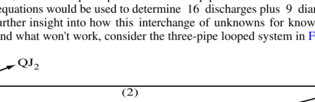
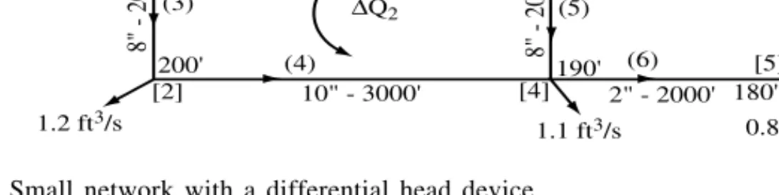
The input data line after DHEAD consists of the following items: (1) the pipe with ∆H;. If we specify a larger HGL downstream of a node with a smaller HGL, we must place a differential master device in one of the pipes between these two nodes. To solve the problem for NETWK, the DHEAD command can be used to indicate that pipe 1 contains the differential height device and that the height of the HGL at node 3 should be 180 meters, which is exactly the height of the water surface in the NETWK. storage tank.
The specification of the impossible could be avoided by considering the pump as a second source of supply. The entry line after the DHEAD command consists of (1) pipe 1 containing the pump, (2) an estimate that this pump should deliver approximately 250 ft head, (3) the HGL should be specified on node 3, (4) the source at the end of pipe 7 must be part of the supplemental equation containing the differential height, and (5) the specified HGL height. In this analysis, stick to the requirement, as in (a), that the pump meets all demand.
DEVELOPING A SOLUTION FOR ANY VARIABLES
- LOGIC AND USE OF NETWEQS1
- DATA TO DESCRIBE THE PIPE SYSTEM
- COMBINATIONS THAT CAN NOT BE UNKNOWNS
The meaning of the three input/output units is as follows: IN2 is the input unit for most of the data describing the piping system. When IN2 is not 0 or 5, then a prompt will ask for the name of the file containing the input data. The program calls the SOLVEQ subroutine (see Appendix A) to solve the linear system of equations obtained by applying Newton's method.
Most of the data describing the system is usually placed in a file that will be read into the Fortran IN2 logical unit. For this particular network, the specification of each discharge and requirements QJ2 and QJ3 is equivalent to a specification of the other two discharges. All requests are considered unknown and the headers are as given in the NETWEQS1 input data.