The most important objects for a transport theory are the invariant manifolds for the Poincare map of the homoclinic flow at fixed points, which physically correspond to stagnation points. We use segments of the stable and unstable manifold to define the time-dependent analogue of the spin limits.
List of Tables
Part I
Chapter 1
The stability of forced solitary waves
Forced solitary waves
The range of physical parameters in which the model is derived (see Lee 1985; Wu 1987) is determined by the following estimates. Among the possible solutions of (1.3) for different choices of the forcing P, are soliton-like solutions (s of the form.
The stability of forced solitary waves
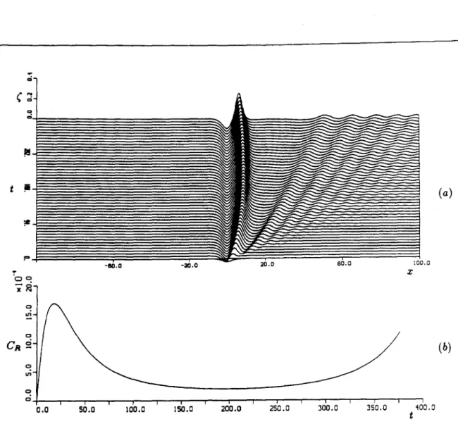
According to the well-known uniqueness property for the initial value problem of the KdV equation on the real line, these steady solitary waves will be solutions of the fKdV equation (1.1), each of which can remain permanently in the form provided. The question of whether these solutions will also have a physical meaning when they are sufficiently perturbed is closely related to their stability properties, and this is the main problem we are currently going to investigate.
Linear stability analysis
- A perturbation expansion for the eigenvalues
- The inner problem for the case of m = 2, µm = m 2 = 4 Forµ= 4 + ES we have
- The outer problem for the case ofµ= 4
- Global spectral behaviour
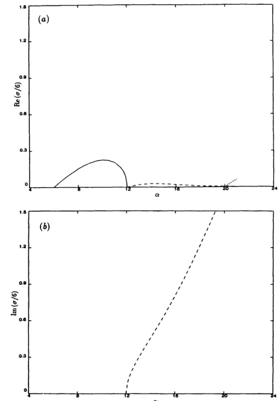
Equation (1.21 ), together with the regularity conditions at infinity for f, constitutes an eigenvalue problem in u, and the stability is determined by the signature of the real part of the eigenvalues, Re u(µ, a) = 0, giving the limit neutral stability in (µ ,a) the room. The instability for µ < 4 is driven by the real part of the eigenvalues according to (1.18), and the previous results show that for subcritical and.
Nonlinear Stability
These are obvious in the sense that they are the ones obtained by Noether's first theorem, due to the invariance of the Lagrangian for equation (1.1) with respect to time. It is interesting to note that an almost identical argument can be made for the nonlinear stability of the stationary solutions of the regularized fKdV equation, which will be used in most of the numerical simulations of Section 1.
Existence of multiple stationary solutions
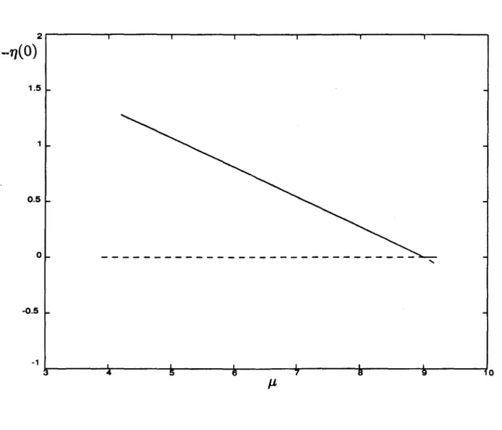
By similar calculations, the solutions that bifurcate at the other two eigenvalues (corresponding to µ = 1 and µ = 9) of the operator I< are. According to the nonlinear stability analysis of Section 1.5., the first question can be answered after evaluating the ground state eigenvalue of the operator I< with the "potential" (s (x) given by one of these stationary solutions.
1. 7 Numerical simulations
Conclusions
We now summarize our results on the stability of stationary solutions of the fKdV equation. Such a wide difference between the real and imaginary parts of the eigenvalue seems to be a characteristic of this class of problems that requires further investigation.
Appendix A
The significance and potential impact of the issues highlighted here deserve continued attention and ongoing investigation. as one can check by the Euler-Lagrange equations,. Now, from the structure of the Lagrangian (A.2), it is clear that we have invariance under the transformation.
Chapter 2
The KdV Model With Boundary Forcing
Introduction
This generalization would lead to consideration of boundary conditions and forcing functions in addition to the appropriately chosen evolution equation. In order to provide some insight for the development of analytical methods for the general case, we investigate the KdV equation in the presence of a boundary forcing, both numerically and exponentially by introducing an approximate method based on the classical inverse scattering transform. This approach is carried out in section 2.3, where the model is described in detail and some comparison with the numerical experiments is presented.
Quite surprisingly, it was found that this new model can provide good qualitative agreement and show some quantitative predictions.
Numerical Results
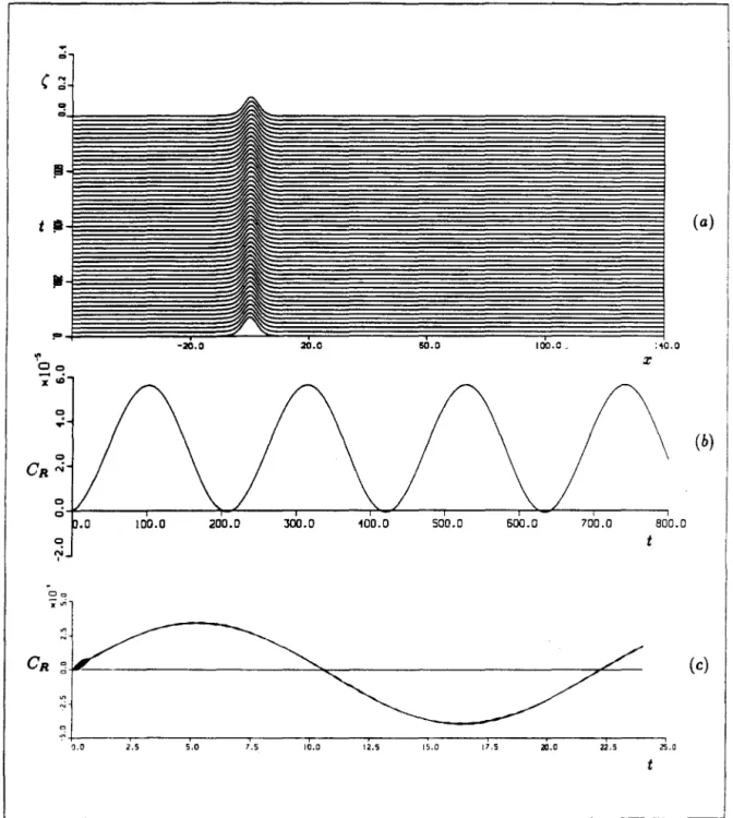
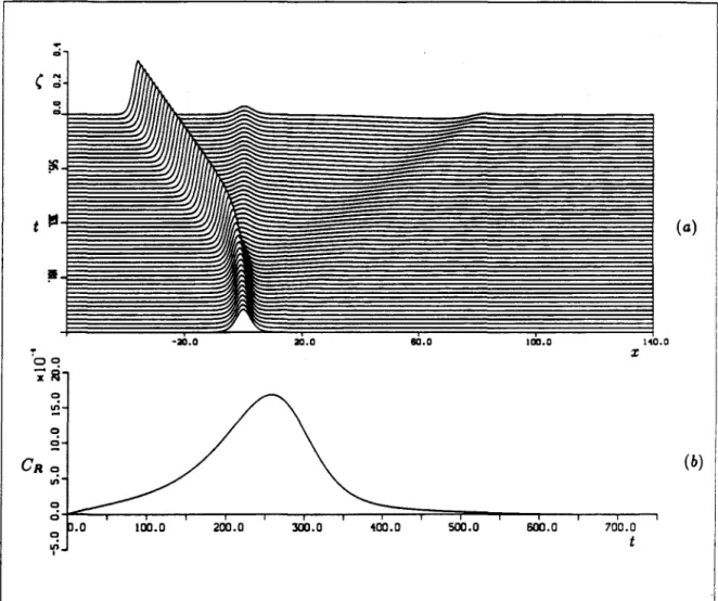
When the forcing is turned off at t, the growth of the wave at the boundary stops, as is clearly seen in the result for t = 0. Then, as soon as time reaches t = 1, this newly formed soliton has already developed so completely that it becomes almost identical to the free soliton of the same amplitude as shown in Figure 2.2. If we take the moment of the first appearance of each relative maximum that appears at the source as the generation time and follow the propagation of these maxima with time, we get the curves in Figures 2.1 b, 2.3b, from which the periodicity of the birth of solitons can be clearly seen.
As expected, the generation of the first soliton occurs sooner and the generation period decreases slightly, compared to the case of T = 0.1 presented in figure 2.1. As shown in figure 2.3c, the soliton speed now approaches the value iUo, which is the speed of a free solitary wave of the same amplitude.
Approximate solutions using 1ST
This agrees well with the numerical calculations for the limiting forcing (2.3) when --+ oo. To compare the results of the current approximate theory with the numerical theories, an appropriate scale for the model must be found. A direct comparison between the estimated IST results and the numerical results is given by Figure 2.11 and Figure 2.12 for cases (2.3) and (2.4), respectively, for the first three solitons.
Direct comparison between the final amplitudes for the first three solitons obtained numerically and those predicted by the approximate 1ST model, for the box-shaped forcing function (2.3). Direct comparison between the final amplitudes for the first three solitons obtained numerically and those predicted by the approximate 1ST model, for the gaussian forcing function (2.4) (Qo = Uo).
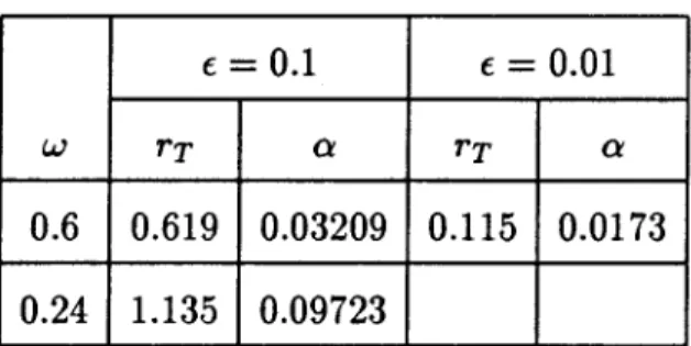
![Figure 2.2. Comparison between the numerical solution at t = l, Uo = 2, T = 0.l, to= 0.25 and the solitary wave solution 12o 2 e- 2 sech 2 [o (z - zo)], o 2 e- 2 = -hx (amplitude), z 0 ~ 0.63](https://thumb-ap.123doks.com/thumbv2/123dok/11010892.0/96.927.112.775.136.821/figure-comparison-numerical-solution-solitary-wave-solution-amplitude.webp)
Part II
CHAOTIC ADVECTION IN A
RAYLEIGH-BENARD FLOW
Chapter 3
The Spreading of Passive Tracer in Chaotic Rayleigh-Benard Flows
Introduction
Our motivation comes from the recent series of experimental studies carried out on transport associated with the Rayleigh-Benard convection. No approach based solely on knowledge of the velocity field would be able to extract information about transport in this case. To model the flow after the onset of the time-dependent instability, we use the stream function introduced by Solomon and Gollub[4] and based on the analysis of Busse[2],[3].
The time dependence will correspond to the collective oscillation of the rolling boundaries in the direction perpendicular to the rolling axes, a phenomenon known as the "equal" oscillatory instability. As an example, we perform some numerical simulation of the time-dependent flow with a term representing the Brownian motion.
The mathematical model and transport theory
- The basic structures governing roll to roll transport
- The spreading of tracer initially contained in one roll
- Chaotic fluid particle motion
- The structures and transport within a roll
This is the crucial observation for the construction of a theory of transport[12] based on the dynamics of the lobes. In the next section, we examine some of the consequences of intersections between manifolds from different tangles. Having introduced the necessary definitions, we now provide the estimate of the length of the turnstile lobe.
As we have seen, these parameters can be even more important than the perturbation strength. A qualitative comparison between visual observations of the roll interface in a time-dependent experiment [4] by Solomon and Gollub [5] and lobe structures for.
Numerical simulations for three "canonical" cases
- Roll concentration of tracer and comparison with a Markov chain model
- The effects of molecular diffusivity
We typically find errors in the most significant digit for some of the patch intersections after 20 iterations. In § 3.3.2 we show how to derive a formula for the measure of the transport region, and discuss the mixing of the tracer in a particular situation. This is contrary to the hope that small patch areas would be the optimal situation for the applicability of the Markov chain approach[.
On the other hand, it is not clear how the direct approach for evaluating the transport region can be improved. This is consistent with the prediction for the measure of the transport region presented by the series method (3.53), which is worse for case (iii).
Acknowledgements
For the rolls not adjacent to R1, the invading tracer will almost exclusively be that propagating via lobes, as the spread by diffusion develops on a slower time scale. However, as the volume of liquid corresponding to a lobe is stretched through regions of clear liquid and the interface is extended, its net tracer content will be reduced by molecular diffusion. In those cases where the turnstiie ioben is small as in (iii), the fluid corresponding to a lobe will be practically depleted of tracer in a few iterations and will enter the distant lobes practically as clear liquid, effectively inhibits the lateral spread of dye.
Appendix B
Therefore, in cases where the turnstile iobe is small as in (iii), the fluid corresponding to a lobe will in a few iterations be virtually devoid of tracer, and enter the distant lobes virtually as clear fluid, effectively inhibiting the lateral spread of dye. be performed numerically, and of those a) is certainly the most expensive in terms of CPU time (see §3). In the following, for clarity and without loss of generality, we will assume that j is an even negative integer or zero. In the following, Sf;, S:T) will denote the reflection operators with respect to the x = 0 and z = ½-axis respectively, sr:r: de.
As usual, using (3.6), the entanglement corresponding to the undisturbed position x = ½ can be obtained from the one for Pt by reflection S;1' and translation SI'". Thanks to these relations, two of the four terms in ( 3.9) involving images of L0 ,1 can be eliminated in favor of terms containing only L1 ,0, which again can be obtained by looking at how the kernel defining the turnstile lobes mapped by P and SI} becomes B.15) .
Appendix C
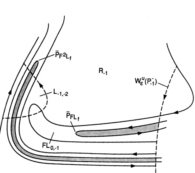
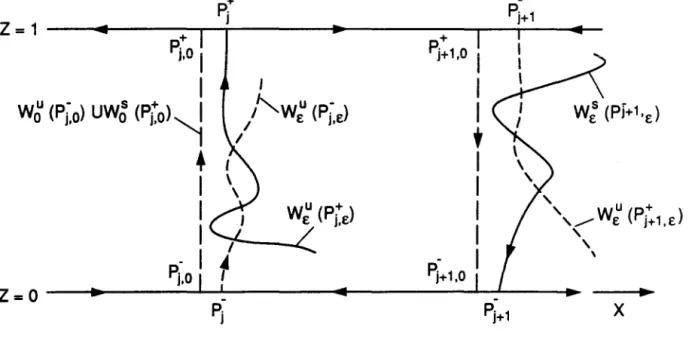
We will refer to the set of points which reach the limits z = 0, z = l asymptotically with forward or backward iteration of the Poincare map as stable central manifold and unstable central manifold respectively[19]. The Jacobian of the vector field (3.2) at the fixed points pf,0 vanishes identically, and information on the local behavior of the invariant manifolds can no longer be obtained by linearizing the vector field around the fixed points. Since aq;••(t,r) j satisfies the first one. C.7) and the integrand can be recognized as that which appears in the Melnikov function (3.20).
In the hyperbolic case this can always be shown to be true[15], but, as already noted, in the present case the convergence of q0(t) to the fixed points is only algebraic. The tangle of the stable (solid) and unstable (dashed) manifold of points Pci and Po, respectively, for the Poincaré section t0 = 0.
PLu,s
Schematic diagram showing the mapping geometry of two rectangular regions B+ and B- to each other. Distribution of escape times for fluid particles in a roll from n = l (red) ton= 100 (blue). Comparison between the exact result (solid) and the Markov model prediction (dashed) for roll j content of species R1 vs .
Comparison between exact (solid) and those simulating numerical diffusivity (dashed) results for roll j content of R1 species vs.