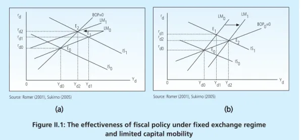
Equation (II.3) shows that BOP = 0 for various combinations of domestic income (Y) and their corresponding domestic interest rates (r). When the BOP is steeper than the LM curve, as shown in Figure II.1.(a), the new internal equilibrium (E1) causes a deficit in the BOP, as it lies below the BOP curve. In another case where the BOP curve is flatter than the LM curve, as depicted in Figure II.1.(b), the new internal balance (point E1) shows a surplus in the BOP as it lies above the BOP curve.
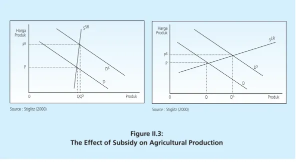
If the BOP curve is steeper than the LM curve, as shown in Figure II.2.(a), fiscal expansionary policies would lead to a deficit in BOP and depress the real exchange rate. If the BOP curve is flatter than the LM curve, as shown in Figure II.2.(b), expansionary fiscal policies would create a surplus in BOP. The left side of equation (II.12) shows the budget deficit and the right side shows the financing sources.
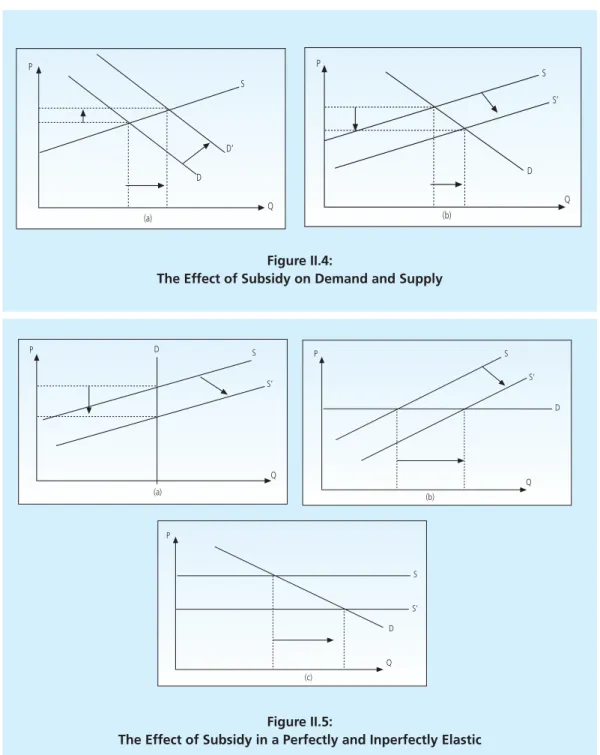
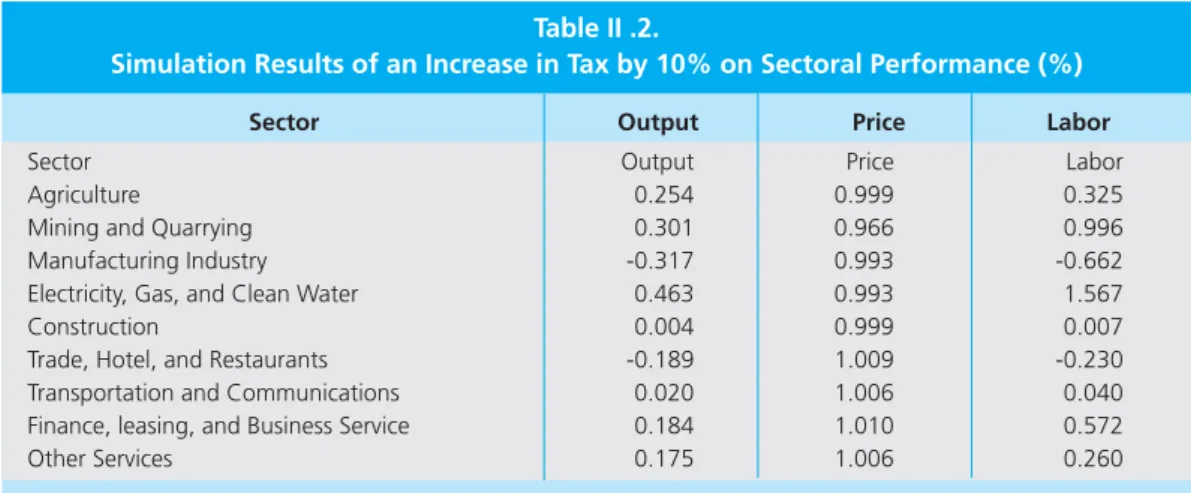
Equation (II.12) shows that the fiscal deficit is equal to the total savings/investment gap from the private sector and the deficit on current items abroad. II.13) (II.14), where Bpf borrows from foreign and private sectors. Equation (II.14) indicates that the deficit on the current accounts abroad is financed by the government's foreign debt and the foreign debt of private individuals. If the demand curve is perfectly inelastic, as shown in Figure II.5 (a), subsidies shift the supply curve from S to S».
If demand is perfectly elastic, as shown in panel (b), Figure II.5, the effect of the subsidy is to increase the equilibrium quantity at the same price.
The effect of government expenditure
This approach views poverty as the inability of the economy to meet the basic needs for food and non-food, as measured by household expenditure. Number of employees, which are the people living below the poverty line, the poverty depth index (P1) and the poverty severity index (P2) can be calculated. The method used is computing poverty line, consists of two components, they are the food poverty line (GKM) and the non-food poverty line.
Poverty line measures are calculated separately for urban and rural areas for each province. The food poverty threshold is the value of expenditure on the minimum need for food, which corresponds to 2100 kilocalories per capita per day. The basic necessities basket consists of 52 items, including rice, fish, meat, eggs, milk, vegetables, beans, fruit and oil.
METHODOLOGY
- Poverty Measurement and Income Distribution
- Production Activity and Factor Market
- Institution
- Commodity Market
- Macroeconomic Balances
- Model Equation
The data obtained, whether from the estimate or the results of the previous studies, are validated or tested for their consistency, therefore considered relevant. The distribution function as shown in equation (II.21) is used to evaluate poverty incidence in each group of households in the general equilibrium economy model. If the average of income is ψ, the income in each household in the group increases by ψ.
The above procedure allows us to compare the degree of poverty generated in the post- and pre-simulation period using the measure developed by Foster, Greer and Thorbecke (F-G-T), Pa. The measure of the poverty line as shown in the monetary poverty line equation (II.24 ) is determined endogenously in the CGE model. It is assumed that the poverty line determined by the basket of goods indicates the consumption of basic needs.
Since the commodity price is determined endogenously in the model, the nominal value of this basket is the poverty line. If the rise in the price of a commodity is due to an external shock, then the poverty line, z, would increase (shifted to the right) and so would poverty, ceteris paribus. In the CGE model, institutions consist of household, business, government, and the rest of the world (RoW).
Total market demand is the sum of domestically produced output and direct imports. The assumption of imperfect transformability (between exports and domestic sales) and imperfect substitutability (between imports and domestic output sold domestically) makes this model relatively better able to capture the empirical realities of most countries. For the government balance, closing used is government savings that remain flexible while all taxes are fixed.
Public consumption is also fixed, either in real terms or as a share of nominal absorption. In order to maintain the same level of real initial investment, the level of savings in the base year of the non-governmental institution is adjusted at one point in time by the same percentage amount. The combination of these three closures in the macro-closure literature is known as Johansen Closures.
In summary, the closures used in this study are (i) government savings are fixed as well as direct taxes (ii) the foreign savings are fixed while the exchange rate is flexible, (iii) the capital establishment is fixed as well as the real investment amount. The equation in the model is divided into four blocks, namely price, production and trade, institutions and obstacle systems.
RESULT AND DISCUSSION
- The Impact of Contraction and Expansion of Fiscal Policy on Indonesian Macro Economic Performance
- The Impact of an Increase in Tax on Economic Performance
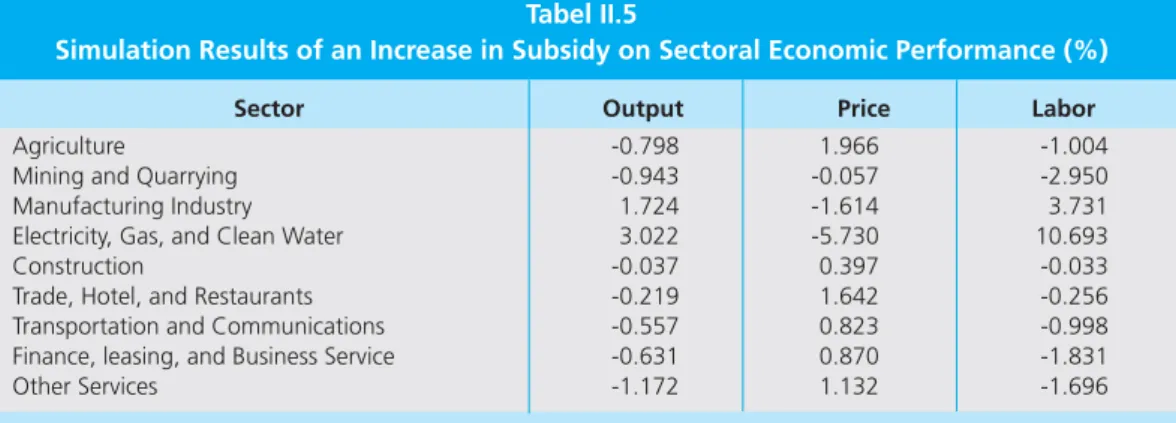
- The Impact of an Increase in Subsidy on Economic Performance
- The Impact of Income Transfer Policy on Indonesia Economic Performance This section describes the simulation results of government policy to increase transfer of
- The Impact of Fiscal Contraction and Expansion Policy on Income Distribution
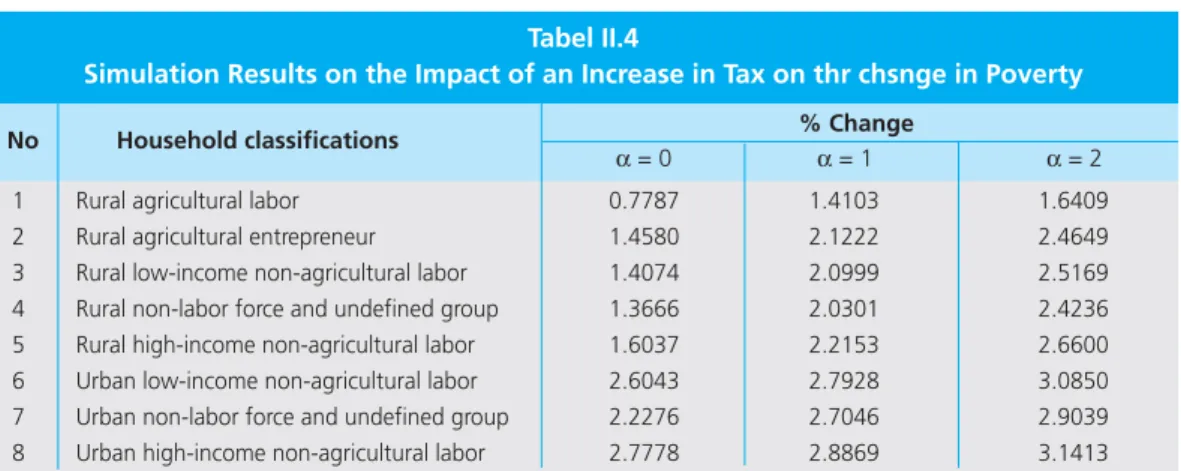
Manufacturing and trade, hotel and restaurants show a negative impact of an increase in tax on output performance. Therefore, their demand for labor also falls as a result of a tax increase. The next effort is to analyze the impact of a 10 percent tax increase on household utility, income, and spending.
The results show that the effect of an increase in tax on utility varies depending on the classification of households. An increase in tax has a negative impact on real income for all groups of households. An increase in tax is expected to affect the poverty ratio index (number of indices or poverty incidence), poverty gap (poverty depth) and poverty intensity index (poverty rate) for households.
In general, the impact of a tax increase on the poverty rate is greater for households in urban areas than for households in rural areas. Simulation results on the impact of a tax increase on poverty reduction. This section examines the impact of an increase in the subsidy on the economic performance of a sector. Using a government simulation, the subsidy increases by 10 percent.
The effect of an increase in the subsidy on the economic performance of the sector The simulation results of a 10 percent increase in the subsidy on production, price and demand for labor are shown in Table II.5. Simulation Results of a subsidy increase on utility and household income (%) The impact of a subsidy increase shows a different picture on the output price. This subsection discusses the simulation results of a 10 percent increase in subsidy on income and household poverty as shown in Table II.6.
An increase in government subsidy has been found to have a positive effect on household income. These three indicators of poverty show a downward trend due to an increase in subsidy (Table II.7). The impact of current transfers on sectoral economic performance An increase in current transfers worth Rp.
It is found that the increase in income transfer has reduced the incidence of poverty among rural households. On the other hand, a tax increase affects the greater inequality of income distribution.

SUMMARY
However, the effects of an increase in taxes, subsidies and current transfers to other household groups are relatively insignificant for changes in income distribution. Center for the Study of African Economies/CSAE, Nuffield College (Oxford University) and CREFA, Canada: Universite Laval. The impact of fiscal policy on income distribution and poverty: a computable global equilibrium approach for Indonesia.
Income distribution, measures of poverty, and trade shocks: A computable general equilibrium model of the developing country archetype. Measuring Poverty and Inequality in a Computable General Equilibrium ModelΔ, Working Paper 99-20, CREFA, Université Laval Departemen Keuangan RI.
APPENDIX