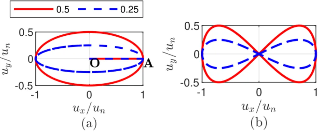
The FDCs of the biaxial model were verified by comparison with FE and smoothed particle hydrodynamic (SPH) simulations for different loading patterns: cyclic uniaxial, 0-shape, 8-shape and transient loading. The parametric study shows that SIFs of buried structures in elastic half-space depend primarily on excitation frequency, shear modulus and Poisson's ratio of the half-space, burial depth and radius of the structure.
Introduction
- Pipelines and seismic actions
- Methods for soil-pipe interaction analysis
- Model neglecting soil-pipe interaction
- Beam-on-Winkler-foundation model considering soil-pipe inter- action
- Challenges in soil-pipe interaction analysis
- Organization of the text
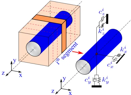
In this method, accurate estimation of the spring stiffness and damping coefficient of the damper is a top priority, which significantly influences the calculation of the internal loads and the design of the spring. This simplified method can account for the true smooth nonlinearity, hysteresis loop, pinch phenomenon and coupling between lateral and vertical ground pipe motions of the ground spring FDC.
Smooth nonlinear hysteresis model for coupled biaxial soil-pipe interaction in sandy soils
Introduction
Most previous work has been based on the assumption of a linear or elastic-perfectly plastic idealization of the true nonlinear FDC. The approach presented here is capable of simulating true nonlinear FDC, soil reaction force hysteresis under dynamic cyclic loading, buckling effects.
Uniaxial hysteresis model
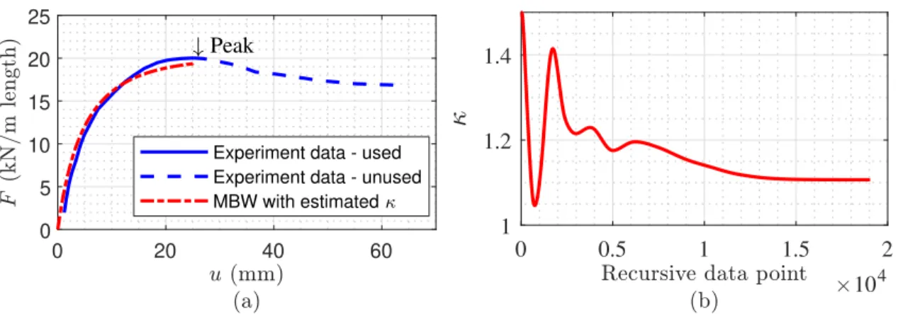
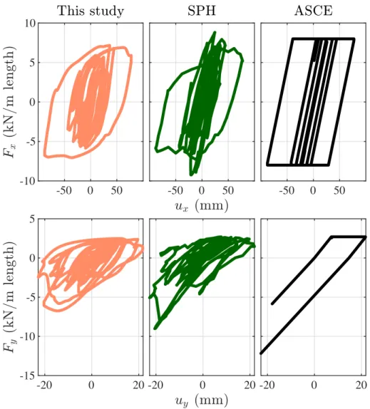
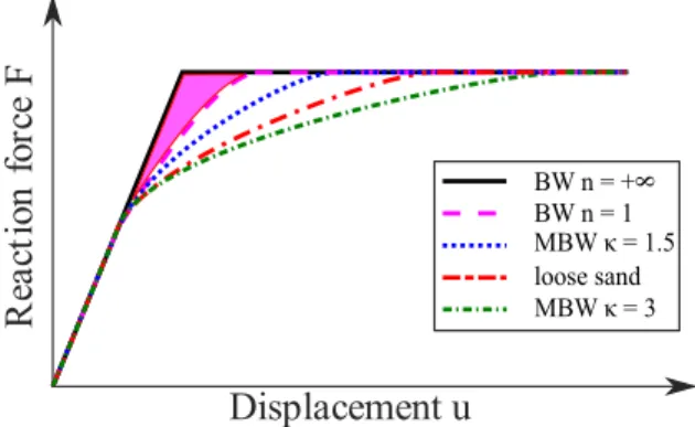
Finally, in Section 2.4, the results of the biaxial model are verified by comparison with the finite element method (FEM), SPH simulations and the BNWF method with elastic-perfectly plastic soil springs calculated according to ASCE(1984) guidelines. In this example, the estimated value𝜅 = 1.1 was used in MBW to generate the FDC and confirm the excellent fit of the experimental data to the idealized MBW model with estimated parameter𝜅, as shown in Fig.2.3(a).
Biaxial hysteresis model
For branch CD of the FDC, the pipe continues to move downward and touches the ground below, which now has stiffness 𝐾𝑦2. The cross stiffness component𝑐 𝑓𝜁sin𝜓 represents the directional difference between d®𝐹 (d®𝜁) and d®𝑢 due to the formation of a plastic zone, assuming that before the first loading (under geostatic stress), the soil stiffness and strength are isotropic .

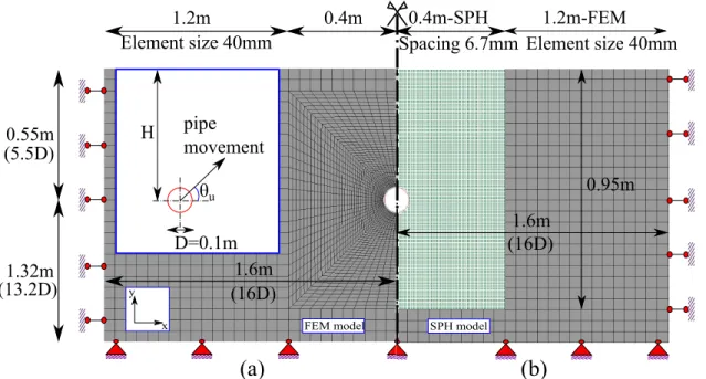
Numerical verification
- Finite element method
- Smoothed-particle hydrodynamics
- Validation of the FEM and SPH models
- Parameter calibration for BMBW model
- Uniaxial cyclic loading
- Suggestions for input parameters
The envelope of the proposed BMBW method was close to that of the FEM simulations. The reaction force of the soil acting on the pipe was investigated for the case of biaxial transient loading.
Conclusions
Despite some limitations, namely the applicability to a rigid (or near-rigid) pipe, and the inability to capture the post-peak behavior of FDC, this study is a first step towards constructing a reduced-order 3D hysteresis model to incorporate floor springs along the lateral, vertical and longitudinal directions of pipeline interaction models - the floor.
Dynamic axial soil impedance function for rigid circular structures buried in elastic half-space
Introduction
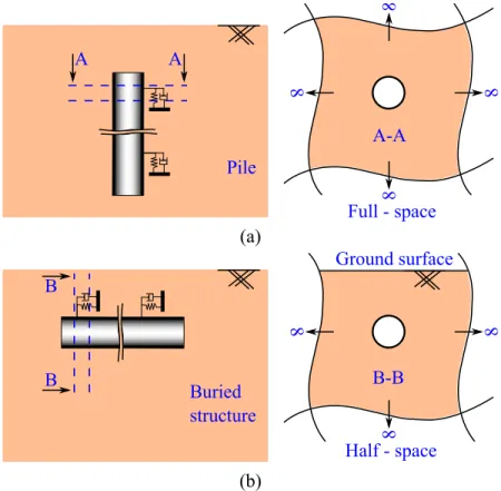
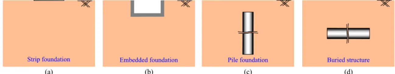
Nevertheless, the SIFs for spatially distributed buried structures (Fig. 3.1d) have not been properly addressed until now, even in the current guidelines of the American Society of Civil Engineers (ASCE, 1984), American Lifeline Alliance (ALA, 2005) . , European Committee for Standardization (CEN, 2006) and Pipeline Research Council International (PRCI, 2009). Furthermore, the relatively high stiffness of the structure compared to the near-surface soil (which is usually soft soil) makes the assumption of rigid buried structures more appropriate. The remainder of this chapter is organized as follows: In Section 3.2, we reviewed some basic principles of SIF.
Review of axial soil impedance function
Finally, we performed parametric studies to investigate the effects of cylinder burial depth and material contrast on the SIF of homogeneous and two-layer half-space. In Section 3.4, we also described the FE modeling procedure to generate SIFs for homogeneous and two-layer half-spaces. Sections 3.6 and 3.7 present SIF and the effect of cylinder burial depth on SIF in the case of a homogeneous and two-layer half-space, respectively.
Analytical solution for soil impedance function of ho- mogeneous half-space
- Assumptions
- Governing equation
- Solution
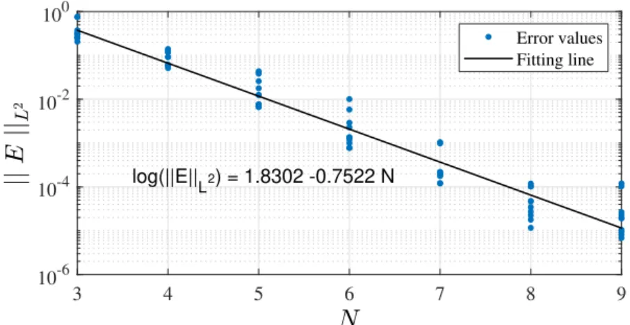
- Truncation errors
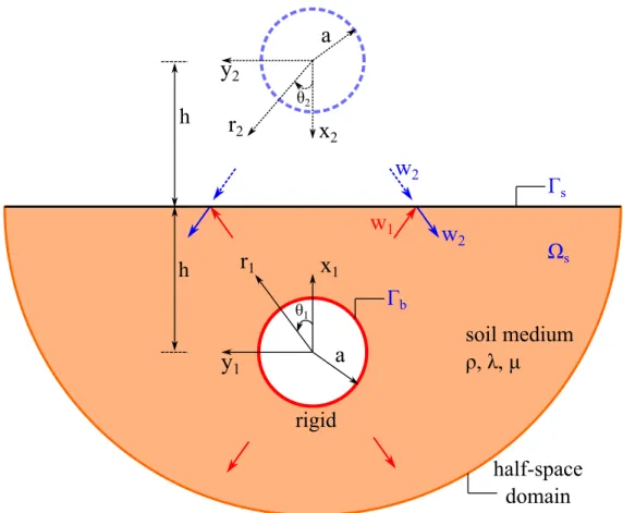
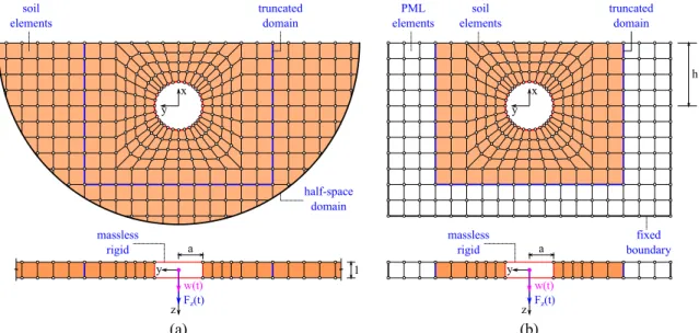
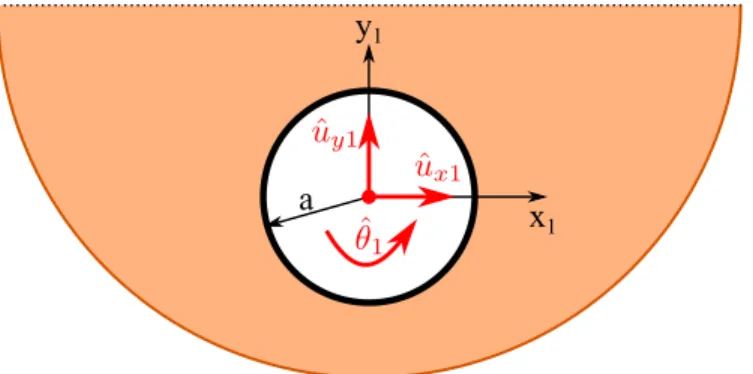
To find the axial impedance, a uniform displacement is imposed on Γ𝑏, which is the circumference of the rigid cylinder, along the direction z 𝑤 = 𝑒𝑖𝜔𝑡. Solving this system of equations yields the complex coefficients 𝐴𝑚 and 𝐵𝑚 to uniquely prescribe the soil domain displacement field via Eq. The degree of convergence of the solutions was tested by solving the problem with different values of 𝑁.
Finite element analysis for soil impedance functions of homogeneous and two-layered half-spaces
- Numerical computation of impedance function
- Finite element models .1 Input time signal.1Input time signal
- Spatial-temporal discretization
If the termination time is short, the signal (at a later time) of the reflected waves cannot be recorded, so some energy from the frequency spectrum is removed. This in turn will lead to disparities in the frequency content of the displacement signal. While Fig.3.10(b) illustrates the frequency domain of the displacement signals, which are truncated at 1.0, 1.5 and 2.0 sec. from the original displacement signal.
Verification
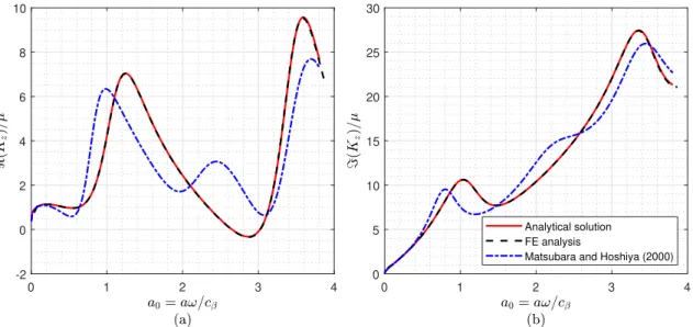
This discrepancy is understandable because Matsubara and Hoshiya solved the problem with the Neumann boundary condition by applying shear stress at the soil-cylinder interface, instead of the Dirichlet boundary condition as done in this work. Due to the averaging nature, their solution may give reasonable SIF under low-frequency loading, but inaccurate SIF under high-frequency excitations. Therefore, the results of Matsubara and Hoshiya coincide with the proposed analytical solutions and FE analysis, as shown in Fig.3.11 and 3.12.
Homogeneous half-space
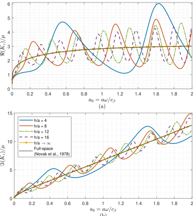
It is noticeable that the preceding patterns of variation of the oscillation amplitude and frequency appear in the real and imaginary parts of the SIF. It is clear that the differences between the SIF of the half-space domain and the full-space domain are significant. As shown in Figure 3.13, the half-space SIFs when ℎ/𝑎→ ∞ perfectly match the full-space SIFs.
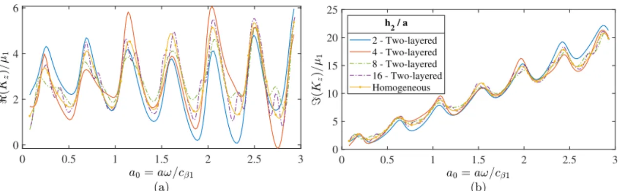
Two-layered half-space
- Effect of material contrast
- Effect of structure location
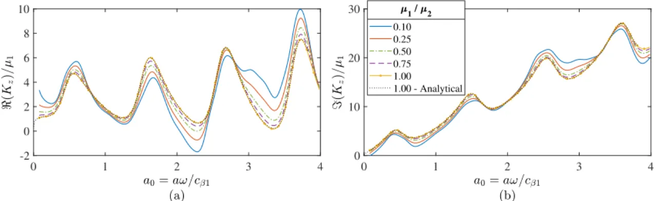
As 𝜇1/𝜇2 becomes larger and approaches 1, the energy trapping becomes smaller and completely escapes from the upper soil layer, the SIF of the two-layer domain finally coincides with that of the homogeneous half-space. In the two-layer domain problem, the dimensionless region A of the SIF curve is defined as. When ℎ2/𝑎 = 16, the SIFs of the two-layer domains oscillate with the highest frequency but the lowest amplitude around the SIF of the corresponding homogeneous half-space.
Conclusions
The SIFs of the homogeneous half-space fluctuate around the SIFs of the homogeneous full space due to reflection from the free surface. Similarly, the SIFs of the bilayer half-space oscillate around the SIFs of the corresponding homogeneous half-space due to reflection from the be- interface. If 𝜇1/𝜇2 ≥ 0.50 or ℎ2/𝑎 ≥ 16, the SIFs of the two-layer half-space can be replaced by those of the corresponding homogeneous half-space for practical design purposes.
Dynamic in-plane soil impedance functions for rigid circular structures buried in elastic
Introduction
To complement the results in three-dimensional space, this chapter examines in-plane dynamic SIFs. In this chapter, we derive an analytical solution for dynamic SIFs in the plane of an infinitely long rigid cylinder buried in a homogeneous elastic half-space. In Section 4.4, we also described the FE modeling procedure for generating dynamic planar SIFs for homogeneous and two-layer half-spaces.
Review of in-plane soil impedance functions
The rest of this chapter is structured as follows: In section 4.2 we discussed some basics of the dynamic in-plane SIFs. 𝑭ˆ(𝜔) =Kˆ (𝜔)𝒖(ˆ 𝜔), (4.1) where 𝜔 ∈ Ris is the angular frequency, 𝑭(ˆ 𝜔) is the applied force vector, Kˆ (𝜔) is the soil impedance matrix, and 𝒖(ˆ 𝜔) is the displacement vector in the center of gravity of the cylinder. Each component of the symmetrical impedance matrix Kˆ (𝜔) is a complex-valued function, where the real part represents the inertia and stiffness, while the imaginary part represents the radiative and material attenuation of the soil domain (Gazetas,1983).
Analytical solution for soil impedance functions of ho- mogeneous half-space
- Assumptions
- Governing equation
- Displacement potentials
- Dirichlet boundary condition at cylinder interface
- Calculation of in-plane soil impedance functions The stresses in the soil domain are computed asThe stresses in the soil domain are computed as
- Integration contour
- Direct evaluation of the integral
- Truncation errors
The characteristic length 𝑎, i.e. the outer radius of the cylinder, is used to normalize ˆ𝑀 and ˆ𝜃1, which indicate the moment and the angle of rotation relative to the center of gravity of the cylinder. The presence of the buried cylinder results in P and SV waves scattering from the structure interface. By solving this system of equations, we uniquely determine the shear and stress fields in the soil domain.
Finite element analysis for soil impedance functions of homogeneous and two-layered half-spaces
- Finite element models
- Input signal for time domain analyses
- Spatial-temporal discretization
To achieve SIF over a wide frequency range, the energy of the input force (or moment) signal must be distributed over the corresponding frequency band. The minimum wavelength is calculated as 𝜆𝑚𝑖𝑛 = 𝑐𝛽/𝑓𝑚 𝑎𝑥, where 𝑓𝑚 𝑎𝑥 is the highest frequency of the signal of interest. In addition, the sampling rate of discrete displacements computed at each time step must be compact enough to capture all of the information of the signal of interest up to the highest frequency.
Verification
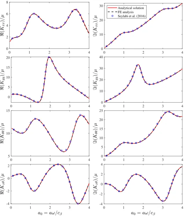
The analytical solution in Section 4.3 and the FE analysis in Section 4.4 for the SIFs for homogeneous half-space were compared with the results of Seylabi et al. It also shows the horizontal impedance𝐾ℎand torsional impedance𝐾𝑡of plane-strain full-space problems, proposed by Novak et al. (1978). When the burial depth is very large, the reflected P and SV waves from the free surface have a negligible effect on the cylinder.
Homogeneous half-space
- Effect of burial depth
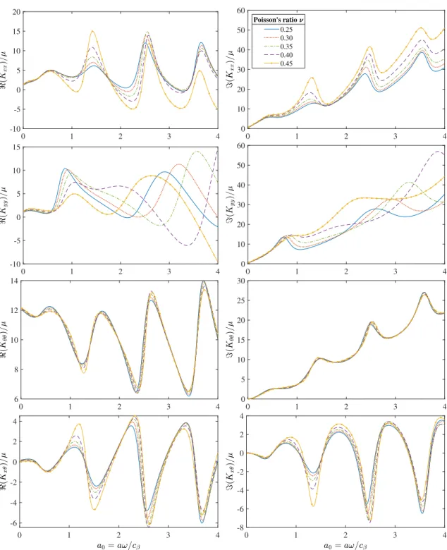
- Effect of Poisson’s ratio
Although the Poisson ratio significantly affects translational impedance, it has virtually no effect on torsional impedance. The translational impedance is largely related to the propagation of a P wave whose velocity is a function of the Poisson ratio. When the frequency is larger, the translation impedance 𝐾𝑥 𝑥 and 𝐾𝑦 𝑦 are more sensitive to the variation of the Poisson ratio compared to the lower frequency case.
Two-layered half-space
- Effect of material contrast
- Effect of structure location
The SIFs of a two-layer domain depend on the burial depth ℎ1, the distance of the cylinder from the interface of the soil layers ℎ2, the Poisson ratio of the soil 𝜈 and the material contrast 𝜇1/𝜇2. For comparison, the SIFs of the corresponding homogeneous half-space with the same ratio ℎ1/𝑎 =4 are also shown. For practical design, the effect of reflected waves from the bottom interface can be negligible, because the SIFs of a two-layer domain and those of the corresponding homogeneous half-space are very similar, especially when ℎ2/𝑎 ≥ 8.
Conclusions
The translational impedance𝐾𝑥 𝑥 and 𝐾𝑦 𝑦 strongly depend on the Poisson ratio of the soil domain, while the torsional impedance 𝐾𝜃 𝜃 hardly does. In the two-layer half-space, all SIF components 𝐾𝑥 𝑥, 𝐾𝑦 𝑦, 𝐾𝜃 𝜃 and 𝐾𝑥 𝜃 deviate from the components of the corresponding homogeneous half-space due to the reflected P- and SV-waves from the soil layer interface. If 𝜇1/𝜇2 ≥ 0.50 or ℎ2/𝑎 ≥ 8, the SIFs of the two-layer half-space can be approximately replaced by those of the corresponding homogeneous half-space for practical design purposes.
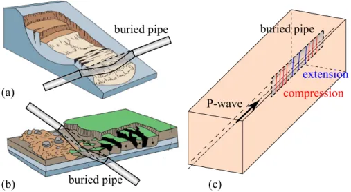
Application: Reduced-order modeling of buried pipe subjected to the propagation of Rayleigh
Introduction
Given the spatial extent of the buried pipeline networks, it is very important to consider the SVEGM in seismic design of such structures to protect the structural integrity. This chapter presents an application of the SIFs derived in Chapters 3 and 4 to build a reduced-order model to analyze the SPI problems. Fig.5.1 illustrates the configuration of the problem, in which a straight pipe is subjected to the propagation of Rayleigh surface wave.
Models for soil-pipe interaction analysis
- Model neglecting soil-pipe interaction
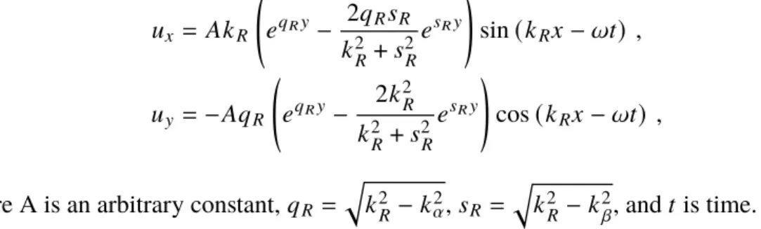
- Rayleigh surface wave in a homogeneous half-space by analytical expression
- Rayleigh surface wave in a heterogeneous half-space by finite element simulation
- Models based on substructure and finite element methods .1 Review of substructure method for soil-structure interaction analysis in case.1Review of substructure method for soil-structure interaction analysis in case
- Soil-pipe interaction model based on substructure method
We used the domain reduction method described by Bielak et al. 2003) to calculate the effective input forces from the predetermined Rayleigh surface wave displacement field of soil 2. Until the early 1970s, many soil-structure interaction models were limited to systems with foundations resting on the surface of a homogeneous half-space and the seismic ground motions being invariant in horizontal planes, e.g. the ground motions of vertically propagating SV waves. Calculation of the foundation input movement (FIM), which is the movement of foundation responsible for the stiffness and geometry of the foundation.
Γ P eff e
Results and comparisons
In general, the results calculated by M2, M3 and M4 are of the same order of magnitude, for both homogeneous and heterogeneous half-spaces. However, there are still some differences in the amplitude of displacement between models M3 and M4, especially in the case of the heterogeneous half-space. Meanwhile, for heterogeneous medium, as shown in Fig.5.15, y-displacements at different control points are significantly different from each other, due to the wave interference inside the basin.
Conclusions
The differences in the displacement patterns between M2 and M3 represent the effect of kinematic interaction, where the existence of a massless pipe bundle changes the ground motions in the free field. For example, the time history of the y-displacement at three control points is fairly uniform for a homogeneous half-space, as shown in Fig. The differential displacement between pipe nodes is known to cause excessive stresses and strains in pipe elements, which can be potentially threatening. the integrity of pipeline networks.
Conclusions
Summary of previous chapters
We showed that the reduced model with appropriate springs and dashpots gives satisfactory results of displacement time histories at the control points compared to those calculated by direct 2D FE analyses. Obviously, this reduced-order model, together with the derived SIFs, provides a robust and versatile tool to improve the analysis of buried structures under seismic excitation while maintaining computational efficiency.
Future work
Bibliography
Ariman (1985), A shell model for buried pipes in earthquakes, International Journal of Soil Dynamics and Earthquake Engineering. Liu (1999), Response of Buried Pipelines Subjected to Earthquake Effects, Multidisciplinary Center for Earthquake Engineering Research, NY. Dakoulas (2010), Finite element analysis of buried steel pipelines under fault displacements, Earth dynamics and earthquake engineering.
Asymptotic method for computing high oscillatory integrals