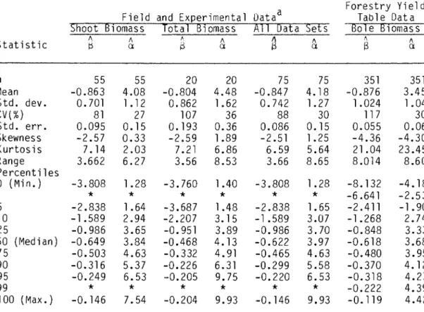
Self-thinning lines from experimental and field data cited by previous authors in support of the. Self-thinning lines from forest yield table data cited by previous authors in support of self-thinning.
RMR 1-3
The self-dilution rule for even-aged plant populations (also called the -3/2 power law or Yoda's law) is reviewed. The evidence does not support acceptance of the self-thinning rule as a quantitative biological law.
CHAPTER 2
The potential ambiguity in the behavior of the model population below the zero isocline can be eliminated as follows. The first two terms of the right-hand side (RHS) of this equation simply give Equation 2.23 for the zero isocline.
The equation associated with the first term on the RHS is simply Equation 2.23 for the zero isocline in the basic model, while the remaining two terms give Where two of the lines cross, the actual zero isocline undergoes a gradual transition from one slope to another.
Density (plants/m 2 )
The slope of the model thinning line is determined only by the power, p, of the area-weight relationship and is equal to the classical thinning line slope of B = -l/2 only when p = 1/3. The position of the self-thinning model line is also affected by the rate constants g0 and m, but these effects are relative.
Density (pI ants/ m 2 )
These effects arise because some of the plant competitors near the edge of the plot extend outside the plot and are not respected. The model was analyzed in three steps: (1) verifying that the dynamics resemble real self-dilution behavior, (2) evaluating variations in the self-dilution trajectory strictly due to. The time required for the density of individuals to drop from an initial value of 10,000 to 1000 was recorded as a measure of the average rate of self-thinning.
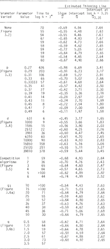
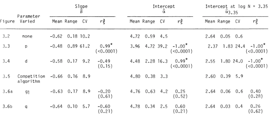
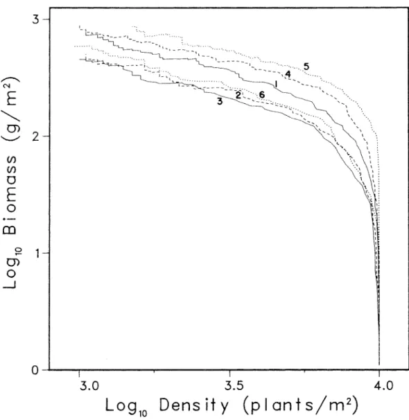
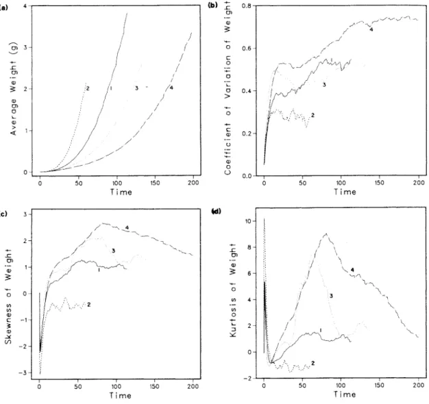
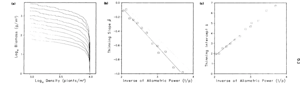
For five of the experiments, the Spearman correlation coefficients, rs, (Sokal and Rohlf 1981) between the experimental parameter and δ, a and a were3.35. calculated and tested for statistical significance to determine whether these thinning descriptors varied systematically with the experimental parameter. Typical dynamic behavior of the simulation model. a) is a log B-log N self-thinning plot, (b) shows the logistic increase in total population biomass, and (c) shows approximately exponential mortality starting with the onset of thinning around time 20. The log B-log N plot of the control group simulations (Figure 3.2) shows that there are variations in the self-thinning trajectory that can only be attributed to persistent effects of the stochastic initial conditions.
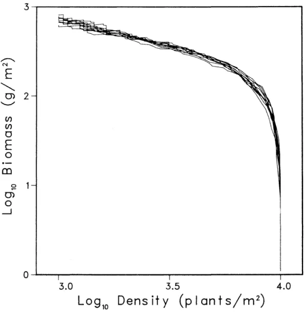
However, the slopes of the self-thinning lines are quite similar and all lines are located within a narrow vertical band. The parameter d, biomass density in the occupied space, influenced the position of the self-dilution line (Figure 3.4a), measured by the dilution cross-section a (rs =0.99, p < 0.0001).
The q = 3.5 simulation was not fitted with a dilution line, as the maximum weight limit came into effect before the linear part of the dilution path was established. Changes in the initial density also did not affect the position of the self-dilution line (Figure 3.6c}). This analysis identified only one parameter, the area related to the strength occupied by a single weight, that affected the self-dilution slope of the model. thinner line.
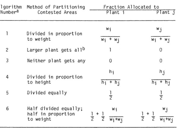
71 . metabolic cost {q and b) affected only the rate of self-thinning, not the slope or position of the thinning line. The important effects of the competition algorithm on the rate of self-thinning and the position of the thinning line are .. significant new results of this analysis. Some results of this analysis are relevant to other theories about the causes of the self-thinning rule.
Three examples of sensitivity of line self-thinning parameters to points selected for analysis. Three examples of the sensitivity of a fitted self-thinning line to points selected for analysis.
Density (pI ants/ m 2)
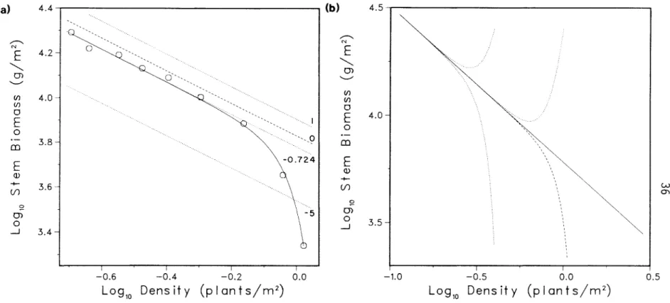
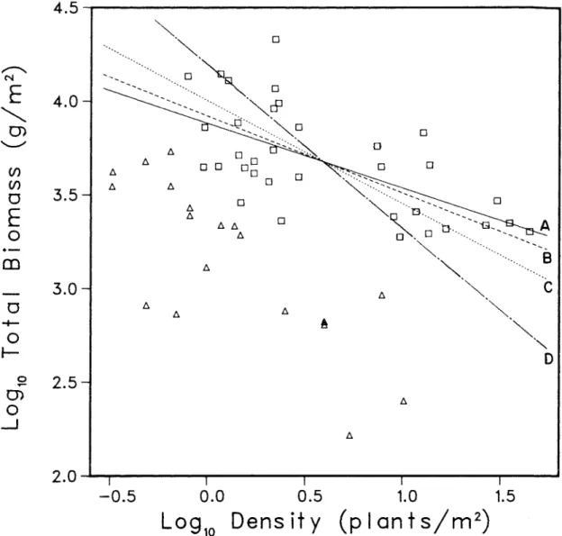
The second shortcoming of the log ~-log N analysis is more serious and damaging to the case for the self-dilution rule: it. The misleading effects of this data transformation are also present in simple plots of the data. The log B-log N plot of the data (Chenopodium album, Yoda et al. 1963) shows an apparent linear constraint which could be estimated by fitting a line through the 13 squared data points in Figure 4.6b.
When the artificial linearity enhancement is removed when inspecting the logarithm B-log N plot for (b), the apparent linear limitation is still apparent; however, many data points fall relatively far from the bounding line (triangles). The log B-log N plot (b) reveals the inadequacy of the straight line model for these data. Evaluation of the self-dilution rule has been hampered by the lack of an objective definition of how close to the predicted value the dilution slope must be to quantitatively match the rule.
A statistical test of the hypothesis that the observed dilution slope equals the predicted value provides a more objective test of agreement with the self-dilution rule. All thinned lines of FYD and 69 (91%) of EFD were estimated by log w to log N association.
CHAPTER 5
Some single-species forest types have been examined in both the EFD and the FYO. For the EFD, the 95% confidence intervals of the thin-line parameters were compared to test for significant differences between the estimates. The predictions of the self-dilution rule are tested here using five different analyses: (l) statistical tests of the.
The statistical tests of the 63 thinning lines reported to demonstrate the self-thinning rule show that this body of evidence does not strongly support the rule. Seventy percent of the thinning lines did show the predicted significant linear relationship between log B and log N, but 32% of the thinning slopes were significantly different from S = -1 and quantitatively disagreed with the thinning rule. In fact, many data sets were too variable to be useful in resolving alternative hypotheses about the slope of the thinner line.
In short, 30% of the datasets showed none. biomass-density relationship, while a further 32% quantitatively disagreed with the -1/2 slope predicted by the thinning rule. The observed slope thinning departures from S = -1/2 for trees in EFO and FYD support Sprugel's (1984).
CHAPTER 6
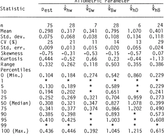
For example, the allometric equation n~w~hw could be suitable for measurements of the average length and average weight of the same stands used to estimate a self-thinning slope. Of the 75 data sets in the EFD that showed significant relationships between log B and log N (chapter 5), 31 had accompanying data sets. Two of the correlations between the transformed thinning slope and the EFD allometric forces were statistically significant.
Histograms of allometric powers of the experimental and field data. a) to (f) show respectively the statistical distributions of the transformed !hinning slope, Pest' and the allometric powers $hw'. Histograms of allometric forces of forestry yield tabular data. a) to (f) show respectively the statistical distributions of the t~ansf~rmed thiQning slope, Pest• and the allometric powers ~hw•. Only in the single case of ~hD in the EFD were the results inconclusive due to the small sample size (n = 6).
Westoby (1976) tested the allometric derivation of the self-thinning rule by measuring the thinning slope of extensive cultivars of Trifolium subterraneum. Several statistically significant relationships between thinning slope and allometric forces were found, but the most predictive only explained 50% of the variation between thinning slopes.
CHAPTER 7
7.2) The shape of plants in a stand can be represented by the ratio between height and radius VOl, T = h/R. R = (TI N)- 112• The estimated R values can then be divided by the reported mean heights to obtain T ranging from 2 to 12 for Gorham•s 65 stands. These two lines define the region of the log w-log N plane, which covers all fully stocked stands equally.
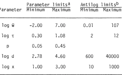
This information was applied to the distribution of ln w by assuming the ninety-ninth. Because ln w is normally distributed, the ninety-ninth percentile value is 4.652 standard deviations above the first percentile value and e4·652a = p. Values of the input parameters log T, p, log d, log w and log p were chosen from uniform random distributions on the.
The volume of any cylinder is a cubic function of the base radius, while the base area is a function of the same radius squared, so that the ratio of these two powers is 3/2. Ranges of variation of variables derived in the Monte Carlo analysis of the improved model.
Density (plants/m 2)
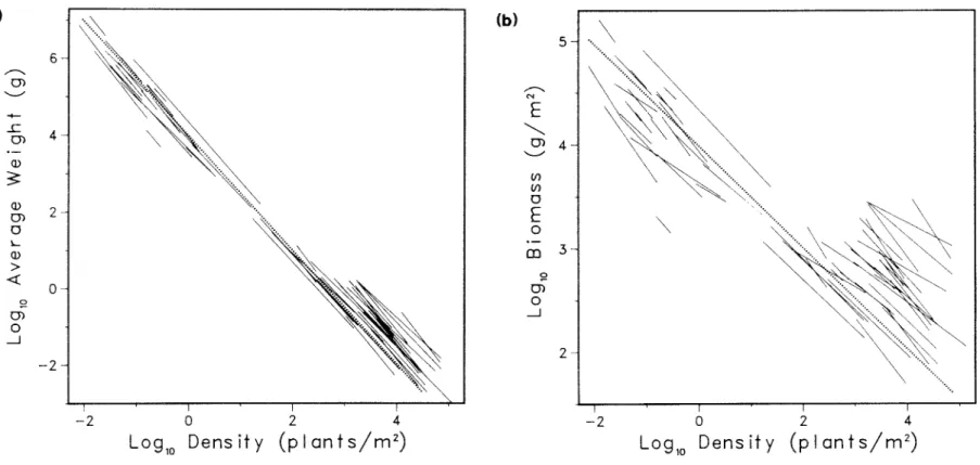
Because different phenomena are examined, the existence of the overall relationship does not provide evidence for or against the self-dilution rule. However, the log B-log N plot of the same data (Figure 7.3b) with the dotted lines encompassing 90% of the observed stands shows that individual, self-thinning lines can vary greatly in slope and position relative to the overall trend and still declining. within the limits of 90%. In fact, the hypothesis that all self-thinning lines are close to log B = -l/2 log N + 4 has been proven before.
Previous analysis of the overall size-density relationship between thinner lines. a) shows 65 previously cited self-thinning lines drawn by applying a reported thinning slope and intercepts (Table A.5) over the range of log N values covered by the thinning line (Table A.3). In (b), the same data and fit are shown in a log B-log N plot, along with dashed lines enclosing 90% of the plant stands. Further verification of the models for the overall relationship can be obtained by comparing the predicted limits of variation.
Considering the extreme simplicity of the model and the rawness of the estimated parameter ranges, the agreement between the predicted range and the range observed for EFD (2.10 ~ log K ~ 5.68) is remarkable. The close agreement between predicted and observed K ranges, despite the crude model parameter estimates, supports the adequacy of the model as a representation of the overall relationship.