Book Info: Presents the most important algorithms and theories that form the core of machine learning. The goal of this textbook is to present the most important algorithms and theories that form the core of machine learning.
CHAPTER
INTRODUCTION
- WELL-POSED LEARNING PROBLEMS
- DESIGNING A LEARNING SYSTEM
- Choosing the Training Experience
- Choosing a Representation for the Target Function
- Choosing a Function Approximation Algorithm
- The Final Design
- PERSPECTIVES AND ISSUES IN MACHINE LEARNING One useful perspective on machine learning is that it involves searching a very
- Issues in Machine Learning
- HOW TO READ THIS BOOK
- SUMMARY AND FURTHER READING
Another important characteristic of the training experience is the degree to which the learner controls the sequence of training examples. What exactly should be the value of the objective function V for a given array state.
CONCEPT LEARNING
GENERAL-TO-SPECIFIC 0,RDERING
INTRODUCTION
Alternatively, each concept can be thought of as a Boolean-valued function defined over this larger set (eg a function defined over all animals, whose value is true for birds and false for other animals). This task is commonly referred to as concept learning, or approximating a Boolean-valued function from examples.
A CONCEPT LEARNING TASK
- Notation
- The Inductive Learning Hypothesis
Given a set of training examples of the target concept c, the problem the learner faces is to hypothesize or estimate c. The symbol H indicates the set of all possible hypotheses that the student can consider regarding the identity of the target concept.
CONCEPT LEARNING AS SEARCH
- General-to-Specific Ordering of Hypotheses
Finally, we will sometimes find the inverse useful and say that h j is more specific than hk when hk is more_general-than h j. As mentioned earlier, hypothesis h2 is more general than hl because any example that satisfies hl also satisfies h2.
FIND-S: FINDING A MAXIMALLY SPECIFIC HYPOTHESIS How can we use the more-general-than partial ordering to organize the search for
Therefore, the hypothesis at each stage is the most specific hypothesis that matches the training examples observed up to this point (hence the name FIND-S). In the event that there are multiple hypotheses that match the training examples, FIND-S will find the most specific one.
VERSION SPACES AND THE CANDIDATE-ELIMINATION ALGORITHM
- Representation
- The LIST-THEN-ELIMINATE Algorithm
- A More Compact Representation for Version Spaces
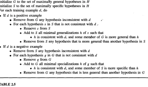
- CANDIDATE-ELIMINATION Learning Algorithm
This is the version space for the Enjoysport concept learning problem and training examples described in Table 2.1. The fourth training example, as shown in Figure 2.6, further generalizes the S-boundary of the version space.
REMARKS ON VERSION SPACES AND CANDIDATE-ELIMINATION .1 Will the CANDIDATE-ELIMINATION Algorithm Converge to the
- What Training Example Should the Learner Request Next?
- How Can Partially Learned Concepts Be Used?
Note that this instance satisfies three of the six hypotheses in the current version space (Figure 2.3). If the trainer classifies this instance as a positive example, the S-bound of the version space can be generalized.
INDUCTIVE BIAS
- A Biased Hypothesis Space
- An Unbiased Learner
- The Futility of Bias-Free Learning
Of course, the inductive bias that is explicitly introduced into the theorem prover is only implicit in the code of the CANDIDATE ELIMINATION algorithm. CANDIDATE ELIMINATION algorithm: New instances are classified only in the case where all members of the current version space agree on the classification.
SUMMARY AND FURTHER READING The main points of this chapter include
The CANDIDATE ELIMINATION algorithm has a stronger inductive bias: that the target concept can be represented in its hypothesis space. The bias associated with the CANDIDATE ELIMINATION algorithm is that the target concept can be found in the provided hypothesis space (c E H).
EXERCISES
Haussler (1988) shows that the size of the general limit can grow exponentially in the number of training examples, even when the hypothesis space consists of simple conjunctions of features. Let us define a new hypothesis space H' consisting of all painful disjunctions of the hypotheses in H.
DECISION TREE LEARNING
INTRODUCTION
DECISION TREE REPRESENTATION
An example is classified by sorting it through the tree to the appropriate leaf node and then returning the classification associated with this leaf (Yes or No in this case). This decision tree classifies Saturday mornings according to whether they are suitable for playing tennis.
APPROPRIATE PROBLEMS FOR DECISION TREE LEARNING Although a variety of decision tree learning methods have been developed with
- Which Attribute Is the Best Classifier?
- ENTROPY MEASURES HOMOGENEITY OF EXAMPLES
- INFORMATION GAIN MEASURES THE EXPECTED REDUCTION IN ENTROPY
- An Illustrative Example
The best attribute is selected and used as a test at the root node of the tree. According to the information acquisition rate, the Outlook attribute provides the best prediction of the target attribute, PlayTennis, compared to the training examples.
HYPOTHESIS SPACE SEARCH IN DECISION TREE LEARNING
The resulting partial decision tree is shown in Figure 3.4, along with the training examples sorted by each new descendant node. The final decision tree that ID3 learned from the 14 training examples of Table 3.2 is shown in Figure 3.1.
INDUCTIVE BIAS IN DECISION TREE LEARNING
- Restriction Biases and Preference Biases
- Why Prefer Short Hypotheses?
Its inductive bias is only a consequence of the ordering of hypotheses from its research strategy. Is ID3's inductive bias favoring shorter decision trees a sound basis for generalization beyond training data.
ISSUES IN DECISION TREE LEARNING
- Avoiding Overfitting the Data
- REDUCED ERROR PRUNING
- RULE POST-PRUNING
- Incorporating Continuous-Valued Attributes
- Alternative Measures for Selecting Attributes
- Handling Attributes with Differing Costs
Predictably, the accuracy of the tree on the training examples increases monotonically as the tree grows. As ID3 adds new nodes to grow the decision tree, the accuracy of the tree measured over the training examples increases monotonically.

SUMMARY AND FURTHER READING The main points of this chapter include
Decision tree post-pruning methods are therefore important to avoid overfitting in decision tree learning (and other inductive reasoning methods that use preference bias). In short, we want to use the ELIMINATE CANDIDATES algorithm to search the hypothesis space of the decision tree.
ARTIFICIAL NEURAL
INTRODUCTION
- Biological Motivation
For example, we consider here ANNs whose individual units produce a single constant value, while biological neurons produce a complex time series of spikes. For more information on attempts to model biological systems using ANNs, see, for example, Churchland and Sejnowski (1992); Zornetzer et al.
NEURAL NETWORK REPRESENTATIONS
The network is shown on the left side of the figure, with the input camera image below. The smaller rectangular chart immediately above the large matrix shows the weights from this hidden unit to each of the 30 output units.
APPROPRIATE PROBLEMS FOR NEURAL NETWORK LEARNING
As can be seen, there are four units that receive input directly from all of the 30 x 32 pixels in the image. The figure on the right shows weight values for one of the hidden units in this network.
PERCEPTRONS
- Representational Power of Perceptrons
- The Perceptron Training Rule
- Gradient Descent and the Delta Rule
- VISUALIZING THE HYPOTHESIS SPACE
- DERIVATION OF THE GRADIENT DESCENT RULE
- STOCHASTIC APPROXIMATION TO GRADIENT DESCENT
- Remarks
Here r] is a positive constant called the learning rate, which determines the step size in gradient descent search. Stochastic gradient descent is repeated over the training examples d in D, at each iteration varying the weights according to the gradient with respect to .

MULTILAYER NETWORKS AND THE BACKPROPAGATION ALGORITHM
- A Differentiable Threshold Unit
- The BACKPROPAGATION Algorithm
- ADDING MOMENTUM
- LEARNING IN ARBITRARY ACYCLIC NETWORKS
- Derivation of the BACKPROPAGATION Rule
1. Insert the instance x' into the network and calculate the output o, of each entity u into the network. Note that the first term on the right side of this equation is just the weight update rule of equation (T4.5) in the BACKPROPAGATION algorithm.
REMARKS ON THE BACKPROPAGATION ALGORITHM .1 Convergence and Local Minima
- Representational Power of Feedforward Networks
- Hypothesis Space Search and Inductive Bias
- Hidden Layer Representations
Every Boolean function can be exactly represented by some network with two layers of units, although the number of hidden units required grows exponentially with the number of network inputs in the worst case. Any function can be approximated to arbitrary precision by a network with three layer units (Cybenko 1988).
- Generalization, Overfitting, and Stopping Criterion
- AN ILLUSTRATIVE EXAMPLE: FACE RECOGNITION
- The Task
- Design Choices
- Learned Hidden Representations
- ADVANCED TOPICS IN ARTIFICIAL NEURAL NETWORKS .1 Alternative Error Functions
- Alternative Error Minimization Procedures
- Recurrent Networks
- Dynamically Modifying Network Structure
- SUMMARY AND FURTHER READING Main points of this chapter include
The evolution of the hidden layer representation can be seen in the second plot of Figure 4.8. Each of these rectangles depicts the weights for one of the four output units in the network (encoding left, straight, right and up).
EVALUATING HYPOTHESES
MOTIVATION
It is therefore important to understand the potential errors inherent in estimating the accuracy of pruned and unpruned trees. First, the observed accuracy of the learned hypothesis on training examples is often a poor estimator of its accuracy on future examples.
ESTIMATING HYPOTHESIS ACCURACY
- Sample Error and True Error
- Confidence Intervals for Discrete-Valued Hypotheses
One is the error rate of the hypothesis on the sample of data available. Given no other information, the best estimate of the true error errorD(h) is the observed sampling error .30.
BASICS OF SAMPLING THEORY
- Error Estimation and Estimating Binomial Proportions
- The Binomial Distribution
- Mean and Variance
- Estimators, Bias, and Variance
- Confidence Intervals
- Two-sided and One-sided Bounds
For sufficiently large values of n, the binomial distribution closely approximates a normal distribution (see Table 5.4) with the same mean and variance. The probability that the random variable R takes on a specific value r (eg, the probability of observing exactly r heads) is given by the Binomial distribution.
A GENERAL APPROACH FOR DERIVING CONFIDENCE INTERVALS
- Central Limit Theorem
This is a rather surprising fact because it states that we know the shape of the distribution that governs the sample mean. Furthermore, the Central Limit Theorem describes how the mean and variance of Y can be used to determine the mean and variance of the individual Y i.
DIFFERENCE IN ERROR OF TWO HYPOTHESES
- Hypothesis Testing
Suppose, for example, that we are interested in the question "what is the probability that error (h1) >. What is the probability that error (hl) > error (h2), given the observed difference in sample errors 2 = . 10 in this case.
COMPARING LEARNING ALGORITHMS
- Paired t Tests
- Practical Considerations
Since d is the mean of the distribution defining 2, this one-sided interval can be equivalently expressed as 2 < p2 + .lo. The above expression describes the expected value of the error difference between the learning methods L A and L B .
SUMMARY AND FURTHER READING The main points of this chapter include
Even with an unbiased estimator, the observed value of the estimator is likely to vary from trial to trial. What is the minimum number of examples you must collect to ensure that the width of the two-sided 95% confidence interval is less than 0.1.
BAYESIAN LEARNING
INTRODUCTION
The second reason that Bayesian methods are important to our study of machine learning is that they provide a useful perspective for understanding many learning algorithms that do not explicitly manipulate probabilities. A practical difficulty in applying Bayesian methods is that they usually require initial knowledge of many probabilities.
BAYES THEOREM
- An Example
We can determine the MAP hypotheses by using Bayes' theorem to calculate the posterior probability of each candidate hypothesis. This step is justified because Bayes' theorem states that the posterior probabilities are just the above quantities divided by the probability of the data, P(@).
BAYES THEOREM AND CONCEPT LEARNING
- Brute-Force Bayes Concept Learning
- MAP Hypotheses and Consistent Learners
In other words, the probability of data D given hypothesis h is 1 if D is consistent with h, and 0 otherwise. To summarize, Bayes' theorem implies that the posterior probability P(h ID) under our assumed P (h) and P(D1h) is.
MAXIMUM LIKELIHOOD AND LEAST-SQUARED ERROR HYPOTHESES
As the above derivation makes clear, the squared error term (di - h) follows directly from the exponent in the definition of the normal distribution. Before we leave our discussion of the relationship between the maximum likelihood hypothesis and the least squares error hypothesis, it is important to to note some limitations of this problem definition.
MAXIMUM LIKELIHOOD HYPOTHESES FOR PREDICTING PROBABILITIES
- Gradient Search to Maximize Likelihood in a Neural Net
Recall that in the maximum likelihood least squares error analysis in the previous section, we made the simplifying assumption that the occurrences (xl. The rule that minimizes cross entropy seeks the maximum likelihood hypothesis under the assumption that the observed Boolean value is a probability). function of the input instance.
MINIMUM DESCRIPTION LENGTH PRINCIPLE
0 -log2 P(D1h) is the description length of the training data D given hypothesis h, under the optimal encoding. The description length of the classifications given the hypothesis is therefore zero in this case.
BAYES OPTIMAL CLASSIFIER
In general, the most likely classification of the new instance is obtained by combining the predictions of all hypotheses, weighted by their posterior probabilities. If the possible classification of the new instance can take any value v j of some set V, then the probability P(vjlD) is that the correct classification for the new instance v; is, fair.
GIBBS ALGORITHM
- An Illustrative Example
- ESTIMATING PROBABILITIES
The naive Bayes classifier is based on the simplifying assumption that the attribute values are conditionally independent given the target value. The naive Bayes classifier thus assigns the target value PlayTennis = no to this new instance, based on the probability estimates learned from the training data.
AN EXAMPLE: LEARNING TO CLASSIFY TEXT
- Experimental Results
In summary, the Naive Bayes VNB classification is a classification that maximizes the probability of observing words that were actually found in The first of these can be easily estimated from the proportion of each class in the training data (P(1ike) = .3 and P(dis1ike) = .7 in the current example).
BAYESIAN BELIEF NETWORKS
- Conditional Independence
- Representation
- Inference
- Learning Bayesian Belief Networks
- Gradient Ascent Training of Bayesian Networks
We define the joint space of the set of variables Y as the cross product V(Yl) x V(Y2) x. The joint probability distribution specifies the probability for each of the possible variable bindings for the tuple (Yl.

