MATHEMATICS FOR
MACHINE LEARNING
Marc Peter Deisenroth A. Aldo Faisal Cheng Soon Ong
MATHEMATICS FOR MACHINE LEARNING DEISENROTH ET AL.
The fundamental mathematical tools needed to understand machine learning include linear algebra, analytic geometry, matrix decompositions, vector calculus, optimization, probability and statistics. These topics are traditionally taught in disparate courses, making it hard for data science or computer science students, or professionals, to effi ciently learn the mathematics. This self-contained textbook bridges the gap between mathematical and machine learning texts, introducing the mathematical concepts with a minimum of prerequisites. It uses these concepts to derive four central machine learning methods: linear regression, principal component analysis, Gaussian mixture models and support vector machines.
For students and others with a mathematical background, these derivations provide a starting point to machine learning texts. For those learning the mathematics for the fi rst time, the methods help build intuition and practical experience with applying mathematical concepts. Every chapter includes worked examples and exercises to test understanding. Programming tutorials are offered on the book’s web site.
MARC PETER DEISENROTH
is Senior Lecturer in Statistical Machine Learning at the Department of Computing, Împerial College London.
A. ALDO FAISAL
leads the Brain & Behaviour Lab at Imperial College London, where he is also Reader in Neurotechnology at the Department of Bioengineering and the Department of Computing.
CHENG SOON ONG
is Principal Research Scientist at the Machine Learning Research Group, Data61, CSIRO. He is also Adjunct Associate Professor at Australian National University.
Deisenrith et al. 9781108455145 Cover. C M Y K
Contents
Foreword 1
Part I Mathematical Foundations 9
1 Introduction and Motivation 11
1.1 Finding Words for Intuitions 12
1.2 Two Ways to Read This Book 13
1.3 Exercises and Feedback 16
2 Linear Algebra 17
2.1 Systems of Linear Equations 19
2.2 Matrices 22
2.3 Solving Systems of Linear Equations 27
2.4 Vector Spaces 35
2.5 Linear Independence 40
2.6 Basis and Rank 44
2.7 Linear Mappings 48
2.8 Affine Spaces 61
2.9 Further Reading 63
Exercises 64
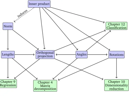
3 Analytic Geometry 70
3.1 Norms 71
3.2 Inner Products 72
3.3 Lengths and Distances 75
3.4 Angles and Orthogonality 76
3.5 Orthonormal Basis 78
3.6 Orthogonal Complement 79
3.7 Inner Product of Functions 80
3.8 Orthogonal Projections 81
3.9 Rotations 91
3.10 Further Reading 94
Exercises 96
4 Matrix Decompositions 98
4.1 Determinant and Trace 99
i
This material is published by Cambridge University Press asMathematics for Machine Learningby
4.2 Eigenvalues and Eigenvectors 105
4.3 Cholesky Decomposition 114
4.4 Eigendecomposition and Diagonalization 115
4.5 Singular Value Decomposition 119
4.6 Matrix Approximation 129
4.7 Matrix Phylogeny 134
4.8 Further Reading 135
Exercises 137
5 Vector Calculus 139
5.1 Differentiation of Univariate Functions 141
5.2 Partial Differentiation and Gradients 146
5.3 Gradients of Vector-Valued Functions 149
5.4 Gradients of Matrices 155
5.5 Useful Identities for Computing Gradients 158
5.6 Backpropagation and Automatic Differentiation 159
5.7 Higher-Order Derivatives 164
5.8 Linearization and Multivariate Taylor Series 165
5.9 Further Reading 170
Exercises 170
6 Probability and Distributions 172
6.1 Construction of a Probability Space 172
6.2 Discrete and Continuous Probabilities 178
6.3 Sum Rule, Product Rule, and Bayes’ Theorem 183
6.4 Summary Statistics and Independence 186
6.5 Gaussian Distribution 197
6.6 Conjugacy and the Exponential Family 205
6.7 Change of Variables/Inverse Transform 214
6.8 Further Reading 221
Exercises 222
7 Continuous Optimization 225
7.1 Optimization Using Gradient Descent 227
7.2 Constrained Optimization and Lagrange Multipliers 233
7.3 Convex Optimization 236
7.4 Further Reading 246
Exercises 247
Part II Central Machine Learning Problems 249
8 When Models Meet Data 251
8.1 Data, Models, and Learning 251
8.2 Empirical Risk Minimization 258
8.3 Parameter Estimation 265
8.4 Probabilistic Modeling and Inference 272
8.5 Directed Graphical Models 278
Contents iii
8.6 Model Selection 283
9 Linear Regression 289
9.1 Problem Formulation 291
9.2 Parameter Estimation 292
9.3 Bayesian Linear Regression 303
9.4 Maximum Likelihood as Orthogonal Projection 313
9.5 Further Reading 315
10 Dimensionality Reduction with Principal Component Analysis 317
10.1 Problem Setting 318
10.2 Maximum Variance Perspective 320
10.3 Projection Perspective 325
10.4 Eigenvector Computation and Low-Rank Approximations 333
10.5 PCA in High Dimensions 335
10.6 Key Steps of PCA in Practice 336
10.7 Latent Variable Perspective 339
10.8 Further Reading 343
11 Density Estimation with Gaussian Mixture Models 348
11.1 Gaussian Mixture Model 349
11.2 Parameter Learning via Maximum Likelihood 350
11.3 EM Algorithm 360
11.4 Latent-Variable Perspective 363
11.5 Further Reading 368
12 Classification with Support Vector Machines 370
12.1 Separating Hyperplanes 372
12.2 Primal Support Vector Machine 374
12.3 Dual Support Vector Machine 383
12.4 Kernels 388
12.5 Numerical Solution 390
12.6 Further Reading 392
References 395
Index 407
Foreword
Machine learning is the latest in a long line of attempts to distill human knowledge and reasoning into a form that is suitable for constructing ma- chines and engineering automated systems. As machine learning becomes more ubiquitous and its software packages become easier to use, it is nat- ural and desirable that the low-level technical details are abstracted away and hidden from the practitioner. However, this brings with it the danger that a practitioner becomes unaware of the design decisions and, hence, the limits of machine learning algorithms.
The enthusiastic practitioner who is interested to learn more about the magic behind successful machine learning algorithms currently faces a daunting set of pre-requisite knowledge:
Programming languages and data analysis tools
Large-scale computation and the associated frameworks
Mathematics and statistics and how machine learning builds on it At universities, introductory courses on machine learning tend to spend early parts of the course covering some of these pre-requisites. For histori- cal reasons, courses in machine learning tend to be taught in the computer science department, where students are often trained in the first two areas of knowledge, but not so much in mathematics and statistics.
Current machine learning textbooks primarily focus on machine learn- ing algorithms and methodologies and assume that the reader is com- petent in mathematics and statistics. Therefore, these books only spend one or two chapters on background mathematics, either at the beginning of the book or as appendices. We have found many people who want to delve into the foundations of basic machine learning methods who strug- gle with the mathematical knowledge required to read a machine learning textbook. Having taught undergraduate and graduate courses at universi- ties, we find that the gap between high school mathematics and the math- ematics level required to read a standard machine learning textbook is too big for many people.
This book brings the mathematical foundations of basic machine learn- ing concepts to the fore and collects the information in a single place so that this skills gap is narrowed or even closed.
1
This material is published by Cambridge University Press asMathematics for Machine Learningby
Why Another Book on Machine Learning?
Machine learning builds upon the language of mathematics to express concepts that seem intuitively obvious but that are surprisingly difficult to formalize. Once formalized properly, we can gain insights into the task we want to solve. One common complaint of students of mathematics around the globe is that the topics covered seem to have little relevance to practical problems. We believe that machine learning is an obvious and direct motivation for people to learn mathematics.
This book is intended to be a guidebook to the vast mathematical lit- erature that forms the foundations of modern machine learning. We mo-
“Math is linked in the popular mind with phobia and anxiety. You’d think we’re discussing spiders.” (Strogatz, 2014, page 281)
tivate the need for mathematical concepts by directly pointing out their usefulness in the context of fundamental machine learning problems. In the interest of keeping the book short, many details and more advanced concepts have been left out. Equipped with the basic concepts presented here, and how they fit into the larger context of machine learning, the reader can find numerous resources for further study, which we provide at the end of the respective chapters. For readers with a mathematical back- ground, this book provides a brief but precisely stated glimpse of machine learning. In contrast to other books that focus on methods and models of machine learning (MacKay, 2003; Bishop, 2006; Alpaydin, 2010; Bar- ber, 2012; Murphy, 2012; Shalev-Shwartz and Ben-David, 2014; Rogers and Girolami, 2016) or programmatic aspects of machine learning (M¨uller and Guido, 2016; Raschka and Mirjalili, 2017; Chollet and Allaire, 2018), we provide only four representative examples of machine learning algo- rithms. Instead, we focus on the mathematical concepts behind the models themselves. We hope that readers will be able to gain a deeper understand- ing of the basic questions in machine learning and connect practical ques- tions arising from the use of machine learning with fundamental choices in the mathematical model.
We do not aim to write a classical machine learning book. Instead, our intention is to provide the mathematical background, applied to four cen- tral machine learning problems, to make it easier to read other machine learning textbooks.
Who Is the Target Audience?
As applications of machine learning become widespread in society, we believe that everybody should have some understanding of its underlying principles. This book is written in an academic mathematical style, which enables us to be precise about the concepts behind machine learning. We encourage readers unfamiliar with this seemingly terse style to persevere and to keep the goals of each topic in mind. We sprinkle comments and remarks throughout the text, in the hope that it provides useful guidance with respect to the big picture.
The book assumes the reader to have mathematical knowledge commonly
Foreword 3 covered in high school mathematics and physics. For example, the reader should have seen derivatives and integrals before, and geometric vectors in two or three dimensions. Starting from there, we generalize these con- cepts. Therefore, the target audience of the book includes undergraduate university students, evening learners and learners participating in online machine learning courses.
In analogy to music, there are three types of interaction that people have with machine learning:
Astute Listener The democratization of machine learning by the pro- vision of open-source software, online tutorials and cloud-based tools al- lows users to not worry about the specifics of pipelines. Users can focus on extracting insights from data using off-the-shelf tools. This enables non- tech-savvy domain experts to benefit from machine learning. This is sim- ilar to listening to music; the user is able to choose and discern between different types of machine learning, and benefits from it. More experi- enced users are like music critics, asking important questions about the application of machine learning in society such as ethics, fairness, and pri- vacy of the individual. We hope that this book provides a foundation for thinking about the certification and risk management of machine learning systems, and allows them to use their domain expertise to build better machine learning systems.
Experienced Artist Skilled practitioners of machine learning can plug and play different tools and libraries into an analysis pipeline. The stereo- typical practitioner would be a data scientist or engineer who understands machine learning interfaces and their use cases, and is able to perform wonderful feats of prediction from data. This is similar to a virtuoso play- ing music, where highly skilled practitioners can bring existing instru- ments to life and bring enjoyment to their audience. Using the mathe- matics presented here as a primer, practitioners would be able to under- stand the benefits and limits of their favorite method, and to extend and generalize existing machine learning algorithms. We hope that this book provides the impetus for more rigorous and principled development of machine learning methods.
Fledgling Composer As machine learning is applied to new domains, developers of machine learning need to develop new methods and extend existing algorithms. They are often researchers who need to understand the mathematical basis of machine learning and uncover relationships be- tween different tasks. This is similar to composers of music who, within the rules and structure of musical theory, create new and amazing pieces.
We hope this book provides a high-level overview of other technical books for people who want to become composers of machine learning. There is a great need in society for new researchers who are able to propose and explore novel approaches for attacking the many challenges of learning from data.
Acknowledgments
We are grateful to many people who looked at early drafts of the book and suffered through painful expositions of concepts. We tried to imple- ment their ideas that we did not vehemently disagree with. We would like to especially acknowledge Christfried Webers for his careful reading of many parts of the book, and his detailed suggestions on structure and presentation. Many friends and colleagues have also been kind enough to provide their time and energy on different versions of each chapter.
We have been lucky to benefit from the generosity of the online commu- nity, who have suggested improvements viahttps://github.com, which greatly improved the book.
The following people have found bugs, proposed clarifications and sug- gested relevant literature, either via https://github.com or personal communication. Their names are sorted alphabetically.
Abdul-Ganiy Usman Adam Gaier
Adele Jackson Aditya Menon Alasdair Tran Aleksandar Krnjaic Alexander Makrigiorgos Alfredo Canziani Ali Shafti
Amr Khalifa Andrew Tanggara Angus Gruen Antal A. Buss
Antoine Toisoul Le Cann Areg Sarvazyan
Artem Artemev Artyom Stepanov Bill Kromydas Bob Williamson Boon Ping Lim Chao Qu Cheng Li Chris Sherlock Christopher Gray Daniel McNamara Daniel Wood Darren Siegel David Johnston Dawei Chen
Ellen Broad
Fengkuangtian Zhu Fiona Condon Georgios Theodorou He Xin
Irene Raissa Kameni Jakub Nabaglo James Hensman Jamie Liu Jean Kaddour Jean-Paul Ebejer Jerry Qiang Jitesh Sindhare John Lloyd Jonas Ngnawe Jon Martin Justin Hsi Kai Arulkumaran Kamil Dreczkowski Lily Wang
Lionel Tondji Ngoupeyou Lydia Kn¨ufing
Mahmoud Aslan Mark Hartenstein Mark van der Wilk Markus Hegland Martin Hewing Matthew Alger Matthew Lee
Foreword 5 Maximus McCann
Mengyan Zhang Michael Bennett Michael Pedersen Minjeong Shin
Mohammad Malekzadeh Naveen Kumar
Nico Montali Oscar Armas Patrick Henriksen Patrick Wieschollek Pattarawat Chormai Paul Kelly
Petros Christodoulou Piotr Januszewski Pranav Subramani Quyu Kong Ragib Zaman Rui Zhang
Ryan-Rhys Griffiths Salomon Kabongo Samuel Ogunmola Sandeep Mavadia Sarvesh Nikumbh Sebastian Raschka
Senanayak Sesh Kumar Karri Seung-Heon Baek
Shahbaz Chaudhary
Shakir Mohamed Shawn Berry
Sheikh Abdul Raheem Ali Sheng Xue
Sridhar Thiagarajan Syed Nouman Hasany Szymon Brych
Thomas B¨uhler Timur Sharapov Tom Melamed Vincent Adam Vincent Dutordoir Vu Minh
Wasim Aftab Wen Zhi
Wojciech Stokowiec Xiaonan Chong Xiaowei Zhang Yazhou Hao Yicheng Luo Young Lee Yu Lu Yun Cheng Yuxiao Huang Zac Cranko Zijian Cao Zoe Nolan
Contributors through GitHub, whose real names were not listed on their GitHub profile, are:
SamDataMad bumptiousmonkey idoamihai
deepakiim
insad HorizonP cs-maillist kudo23
empet victorBigand 17SKYE jessjing1995
We are also very grateful to Parameswaran Raman and the many anony- mous reviewers, organized by Cambridge University Press, who read one or more chapters of earlier versions of the manuscript, and provided con- structive criticism that led to considerable improvements. A special men- tion goes to Dinesh Singh Negi, our LATEX support, for detailed and prompt advice about LATEX-related issues. Last but not least, we are very grateful to our editor Lauren Cowles, who has been patiently guiding us through the gestation process of this book.
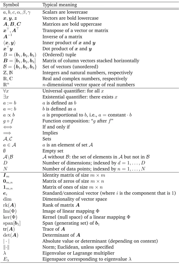
Table of Symbols
Symbol Typical meaning
a, b, c, α, β, γ Scalars are lowercase x,y,z Vectors are bold lowercase A,B,C Matrices are bold uppercase x⊤,A⊤ Transpose of a vector or matrix A−1 Inverse of a matrix
⟨x,y⟩ Inner product ofxandy x⊤y Dot product ofxandy B= (b1,b2,b3) (Ordered) tuple
B= [b1,b2,b3] Matrix of column vectors stacked horizontally B={b1,b2,b3} Set of vectors (unordered)
Z,N Integers and natural numbers, respectively R,C Real and complex numbers, respectively Rn n-dimensional vector space of real numbers
∀x Universal quantifier: for allx
∃x Existential quantifier: there existsx a:=b ais defined asb
a=:b bis defined asa
a∝b ais proportional tob, i.e.,a=constant·b g◦f Function composition: “gafterf”
⇐⇒ If and only if
=⇒ Implies
A,C Sets
a∈ A ais an element of setA
∅ Empty set
A\B AwithoutB: the set of elements inAbut not inB D Number of dimensions; indexed byd= 1, . . . , D N Number of data points; indexed byn= 1, . . . , N Im Identity matrix of sizem×m
0m,n Matrix of zeros of sizem×n 1m,n Matrix of ones of sizem×n
ei Standard/canonical vector (whereiis the component that is1) dim Dimensionality of vector space
rk(A) Rank of matrixA
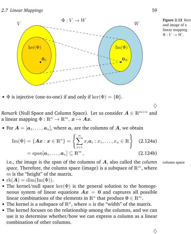
Im(Φ) Image of linear mappingΦ
ker(Φ) Kernel (null space) of a linear mappingΦ span[b1] Span (generating set) ofb1
tr(A) Trace ofA
det(A) Determinant ofA
| · | Absolute value or determinant (depending on context)
∥·∥ Norm; Euclidean, unless specified λ Eigenvalue or Lagrange multiplier
Eλ Eigenspace corresponding to eigenvalueλ
Foreword 7
Symbol Typical meaning
x⊥y Vectorsxandyare orthogonal
V Vector space
V⊥ Orthogonal complement of vector spaceV PN
n=1xn Sum of thexn:x1+. . .+xN
QN
n=1xn Product of thexn:x1·. . .·xN
θ Parameter vector
∂f
∂x Partial derivative off with respect tox
df
dx Total derivative off with respect tox
∇ Gradient
f∗= minxf(x) The smallest function value off
x∗ ∈arg minxf(x) The valuex∗that minimizesf (note:arg minreturns a set of values)
L Lagrangian
L Negative log-likelihood
n k
Binomial coefficient,nchoosek
VX[x] Variance ofxwith respect to the random variableX EX[x] Expectation ofxwith respect to the random variableX CovX,Y[x,y] Covariance betweenxandy.
X⊥⊥Y |Z Xis conditionally independent ofY givenZ X∼p Random variableXis distributed according top N µ,Σ Gaussian distribution with meanµand covarianceΣ Ber(µ) Bernoulli distribution with parameterµ
Bin(N, µ) Binomial distribution with parametersN, µ Beta(α, β) Beta distribution with parametersα, β
Table of Abbreviations and Acronyms Acronym Meaning
e.g. Exempli gratia (Latin: for example) GMM Gaussian mixture model
i.e. Id est (Latin: this means)
i.i.d. Independent, identically distributed MAP Maximum a posteriori
MLE Maximum likelihood estimation/estimator ONB Orthonormal basis
PCA Principal component analysis
PPCA Probabilistic principal component analysis REF Row-echelon form
SPD Symmetric, positive definite SVM Support vector machine
Part I
Mathematical Foundations
9
This material is published by Cambridge University Press asMathematics for Machine Learningby
1
Introduction and Motivation
Machine learning is about designing algorithms that automatically extract valuable information from data. The emphasis here is on “automatic”, i.e., machine learning is concerned about general-purpose methodologies that can be applied to many datasets, while producing something that is mean- ingful. There are three concepts that are at the core of machine learning:
data, a model, and learning.
Since machine learning is inherently data driven, data is at the core data
of machine learning. The goal of machine learning is to design general- purpose methodologies to extract valuable patterns from data, ideally without much domain-specific expertise. For example, given a large corpus of documents (e.g., books in many libraries), machine learning methods can be used to automatically find relevant topics that are shared across documents (Hoffman et al., 2010). To achieve this goal, we designmod-
elsthat are typically related to the process that generates data, similar to model
the dataset we are given. For example, in a regression setting, the model would describe a function that maps inputs to real-valued outputs. To paraphrase Mitchell (1997): A model is said to learn from data if its per- formance on a given task improves after the data is taken into account.
The goal is to find good models that generalize well to yet unseen data,
which we may care about in the future.Learningcan be understood as a learning
way to automatically find patterns and structure in data by optimizing the parameters of the model.
While machine learning has seen many success stories, and software is readily available to design and train rich and flexible machine learning systems, we believe that the mathematical foundations of machine learn- ing are important in order to understand fundamental principles upon which more complicated machine learning systems are built. Understand- ing these principles can facilitate creating new machine learning solutions, understanding and debugging existing approaches, and learning about the inherent assumptions and limitations of the methodologies we are work- ing with.
11
This material is published by Cambridge University Press asMathematics for Machine Learningby
1.1 Finding Words for Intuitions
A challenge we face regularly in machine learning is that concepts and words are slippery, and a particular component of the machine learning system can be abstracted to different mathematical concepts. For example, the word “algorithm” is used in at least two different senses in the con- text of machine learning. In the first sense, we use the phrase “machine learning algorithm” to mean a system that makes predictions based on in- put data. We refer to these algorithms aspredictors. In the second sense,
predictor
we use the exact same phrase “machine learning algorithm” to mean a system that adapts some internal parameters of the predictor so that it performs well on future unseen input data. Here we refer to this adapta- tion astraininga system.
training
This book will not resolve the issue of ambiguity, but we want to high- light upfront that, depending on the context, the same expressions can mean different things. However, we attempt to make the context suffi- ciently clear to reduce the level of ambiguity.
The first part of this book introduces the mathematical concepts and foundations needed to talk about the three main components of a machine learning system: data, models, and learning. We will briefly outline these components here, and we will revisit them again in Chapter 8 once we have discussed the necessary mathematical concepts.
While not all data is numerical, it is often useful to consider data in a number format. In this book, we assume that data has already been appropriately converted into a numerical representation suitable for read- ing into a computer program. Therefore, we think of data as vectors. As
data as vectors
another illustration of how subtle words are, there are (at least) three different ways to think about vectors: a vector as an array of numbers (a computer science view), a vector as an arrow with a direction and magni- tude (a physics view), and a vector as an object that obeys addition and scaling (a mathematical view).
Amodelis typically used to describe a process for generating data, sim-
model
ilar to the dataset at hand. Therefore, good models can also be thought of as simplified versions of the real (unknown) data-generating process, capturing aspects that are relevant for modeling the data and extracting hidden patterns from it. A good model can then be used to predict what would happen in the real world without performing real-world experi- ments.
We now come to the crux of the matter, the learning component of
learning
machine learning. Assume we are given a dataset and a suitable model.
Trainingthe model means to use the data available to optimize some pa- rameters of the model with respect to a utility function that evaluates how well the model predicts the training data. Most training methods can be thought of as an approach analogous to climbing a hill to reach its peak.
In this analogy, the peak of the hill corresponds to a maximum of some
1.2 Two Ways to Read This Book 13 desired performance measure. However, in practice, we are interested in the model to perform well on unseen data. Performing well on data that we have already seen (training data) may only mean that we found a good way to memorize the data. However, this may not generalize well to unseen data, and, in practical applications, we often need to expose our machine learning system to situations that it has not encountered before.
Let us summarize the main concepts of machine learning that we cover in this book:
We represent data as vectors.
We choose an appropriate model, either using the probabilistic or opti- mization view.
We learn from available data by using numerical optimization methods with the aim that the model performs well on data not used for training.
1.2 Two Ways to Read This Book
We can consider two strategies for understanding the mathematics for machine learning:
Bottom-up: Building up the concepts from foundational to more ad- vanced. This is often the preferred approach in more technical fields, such as mathematics. This strategy has the advantage that the reader at all times is able to rely on their previously learned concepts. Unfor- tunately, for a practitioner many of the foundational concepts are not particularly interesting by themselves, and the lack of motivation means that most foundational definitions are quickly forgotten.
Top-down: Drilling down from practical needs to more basic require- ments. This goal-driven approach has the advantage that the readers know at all times why they need to work on a particular concept, and there is a clear path of required knowledge. The downside of this strat- egy is that the knowledge is built on potentially shaky foundations, and the readers have to remember a set of words that they do not have any way of understanding.
We decided to write this book in a modular way to separate foundational (mathematical) concepts from applications so that this book can be read in both ways. The book is split into two parts, where Part I lays the math- ematical foundations and Part II applies the concepts from Part I to a set of fundamental machine learning problems, which form four pillars of machine learning as illustrated in Figure 1.1: regression, dimensionality reduction, density estimation, and classification. Chapters in Part I mostly build upon the previous ones, but it is possible to skip a chapter and work backward if necessary. Chapters in Part II are only loosely coupled and can be read in any order. There are many pointers forward and backward
Figure 1.1 The foundations and four pillars of machine learning.
Classification
Density Estimation
Regression Dimensionality Reduction
Machine Learning
Vector Calculus Probability & Distributions Optimization Analytic Geometry Matrix Decomposition Linear Algebra
between the two parts of the book to link mathematical concepts with machine learning algorithms.
Of course there are more than two ways to read this book.Most readers learn using a combination of top-down and bottom-up approaches, some- times building up basic mathematical skills before attempting more com- plex concepts, but also choosing topics based on applications of machine learning.
Part I Is about Mathematics
The four pillars of machine learning we cover in this book (see Figure 1.1) require a solid mathematical foundation, which is laid out in Part I.
We represent numerical data as vectors and represent a table of such data as a matrix. The study of vectors and matrices is calledlinear algebra, which we introduce in Chapter 2. The collection of vectors as a matrix is
linear algebra
also described there.
Given two vectors representing two objects in the real world, we want to make statements about their similarity. The idea is that vectors that are similar should be predicted to have similar outputs by our machine learning algorithm (our predictor). To formalize the idea of similarity be- tween vectors, we need to introduce operations that take two vectors as input and return a numerical value representing their similarity. The con- struction of similarity and distances is central toanalytic geometryand is
analytic geometry
discussed in Chapter 3.
In Chapter 4, we introduce some fundamental concepts about matri- ces andmatrix decomposition. Some operations on matrices are extremely
matrix
decomposition useful in machine learning, and they allow for an intuitive interpretation of the data and more efficient learning.
We often consider data to be noisy observations of some true underly- ing signal. We hope that by applying machine learning we can identify the signal from the noise. This requires us to have a language for quantify- ing what “noise” means. We often would also like to have predictors that
1.2 Two Ways to Read This Book 15 allow us to express some sort of uncertainty, e.g., to quantify the confi- dence we have about the value of the prediction at a particular test data
point. Quantification of uncertainty is the realm ofprobability theoryand probability theory
is covered in Chapter 6.
To train machine learning models, we typically find parameters that maximize some performance measure. Many optimization techniques re- quire the concept of a gradient, which tells us the direction in which to
search for a solution. Chapter 5 is about vector calculus and details the vector calculus
concept of gradients, which we subsequently use in Chapter 7, where we
talk aboutoptimizationto find maxima/minima of functions. optimization
Part II Is about Machine Learning
The second part of the book introduces four pillars of machine learning as shown in Figure 1.1. We illustrate how the mathematical concepts in- troduced in the first part of the book are the foundation for each pillar.
Broadly speaking, chapters are ordered by difficulty (in ascending order).
In Chapter 8, we restate the three components of machine learning (data, models, and parameter estimation) in a mathematical fashion. In addition, we provide some guidelines for building experimental set-ups that guard against overly optimistic evaluations of machine learning sys- tems. Recall that the goal is to build a predictor that performs well on unseen data.
In Chapter 9, we will have a close look at linear regression, where our linear regression
objective is to find functions that map inputsx∈RDto corresponding ob- served function valuesy∈R, which we can interpret as the labels of their respective inputs. We will discuss classical model fitting (parameter esti- mation) via maximum likelihood and maximum a posteriori estimation, as well as Bayesian linear regression, where we integrate the parameters out instead of optimizing them.
Chapter 10 focuses ondimensionality reduction, the second pillar in Fig- dimensionality reduction
ure 1.1, using principal component analysis. The key objective of dimen- sionality reduction is to find a compact, lower-dimensional representation of high-dimensional datax ∈ RD, which is often easier to analyze than the original data. Unlike regression, dimensionality reduction is only con- cerned about modeling the data – there are no labels associated with a data pointx.
In Chapter 11, we will move to our third pillar:density estimation. The density estimation
objective of density estimation is to find a probability distribution that de- scribes a given dataset. We will focus on Gaussian mixture models for this purpose, and we will discuss an iterative scheme to find the parameters of this model. As in dimensionality reduction, there are no labels associated with the data pointsx∈RD. However, we do not seek a low-dimensional representation of the data. Instead, we are interested in a density model that describes the data.
Chapter 12 concludes the book with an in-depth discussion of the fourth
pillar:classification. We will discuss classification in the context of support
classification
vector machines. Similar to regression (Chapter 9), we have inputsxand corresponding labelsy. However, unlike regression, where the labels were real-valued, the labels in classification are integers, which requires special care.
1.3 Exercises and Feedback
We provide some exercises in Part I, which can be done mostly by pen and paper. For Part II, we provide programming tutorials (jupyter notebooks) to explore some properties of the machine learning algorithms we discuss in this book.
We appreciate that Cambridge University Press strongly supports our aim to democratize education and learning by making this book freely available for download at
https://mml-book.com
where tutorials, errata, and additional materials can be found. Mistakes can be reported and feedback provided using the preceding URL.
2
Linear Algebra
When formalizing intuitive concepts, a common approach is to construct a set of objects (symbols) and a set of rules to manipulate these objects. This
is known as analgebra. Linear algebra is the study of vectors and certain algebra
rules to manipulate vectors. The vectors many of us know from school are called “geometric vectors”, which are usually denoted by a small arrow above the letter, e.g., −→x and−→y. In this book, we discuss more general concepts of vectors and use a bold letter to represent them, e.g.,xandy. In general, vectors are special objects that can be added together and multiplied by scalars to produce another object of the same kind. From an abstract mathematical viewpoint, any object that satisfies these two properties can be considered a vector. Here are some examples of such vector objects:
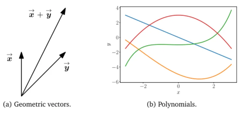
1. Geometric vectors. This example of a vector may be familiar from high school mathematics and physics. Geometric vectors – see Figure 2.1(a) – are directed segments, which can be drawn (at least in two dimen- sions). Two geometric vectors→x, →ycan be added, such that→x+→y=→z is another geometric vector. Furthermore, multiplication by a scalar λ→x,λ∈ R, is also a geometric vector. In fact, it is the original vector scaled by λ. Therefore, geometric vectors are instances of the vector concepts introduced previously. Interpreting vectors as geometric vec- tors enables us to use our intuitions about direction and magnitude to reason about mathematical operations.
2. Polynomials are also vectors; see Figure 2.1(b): Two polynomials can
Figure 2.1 Different types of vectors. Vectors can be surprising objects, including (a) geometric vectors
and (b) polynomials.
→x
→y
→x+→y
(a) Geometric vectors.
−2 0 2
x
−6
−4
−2 0 2 4
y
(b) Polynomials.
17
This material is published by Cambridge University Press asMathematics for Machine Learningby
be added together, which results in another polynomial; and they can be multiplied by a scalar λ ∈ R, and the result is a polynomial as well. Therefore, polynomials are (rather unusual) instances of vectors.
Note that polynomials are very different from geometric vectors. While geometric vectors are concrete “drawings”, polynomials are abstract concepts. However, they are both vectors in the sense previously de- scribed.
3. Audio signals are vectors. Audio signals are represented as a series of numbers. We can add audio signals together, and their sum is a new audio signal. If we scale an audio signal, we also obtain an audio signal.
Therefore, audio signals are a type of vector, too.
4. Elements of Rn (tuples of n real numbers) are vectors. Rn is more abstract than polynomials, and it is the concept we focus on in this book. For instance,
a=
1 2 3
∈R3 (2.1)
is an example of a triplet of numbers. Adding two vectors a,b ∈ Rn component-wise results in another vector:a+b=c∈Rn. Moreover, multiplying a ∈ Rn by λ ∈ R results in a scaled vector λa ∈ Rn. Considering vectors as elements of Rn has an additional benefit that
Be careful to check whether array operations actually perform vector operations when implementing on a computer.
it loosely corresponds to arrays of real numbers on a computer. Many programming languages support array operations, which allow for con- venient implementation of algorithms that involve vector operations.
Linear algebra focuses on the similarities between these vector concepts.
We can add them together and multiply them by scalars. We will largely
Pavel Grinfeld’s series on linear algebra:
http://tinyurl.
com/nahclwm Gilbert Strang’s course on linear algebra:
http://tinyurl.
com/29p5q8j 3Blue1Brown series on linear algebra:
https://tinyurl.
com/h5g4kps
focus on vectors in Rn since most algorithms in linear algebra are for- mulated in Rn. We will see in Chapter 8 that we often consider data to be represented as vectors in Rn. In this book, we will focus on finite- dimensional vector spaces, in which case there is a 1:1 correspondence between any kind of vector andRn. When it is convenient, we will use intuitions about geometric vectors and consider array-based algorithms.
One major idea in mathematics is the idea of “closure”. This is the ques- tion: What is the set of all things that can result from my proposed oper- ations? In the case of vectors: What is the set of vectors that can result by starting with a small set of vectors, and adding them to each other and scaling them? This results in a vector space (Section 2.4). The concept of a vector space and its properties underlie much of machine learning. The concepts introduced in this chapter are summarized in Figure 2.2.
This chapter is mostly based on the lecture notes and books by Drumm and Weil (2001), Strang (2003), Hogben (2013), Liesen and Mehrmann (2015), as well as Pavel Grinfeld’s Linear Algebra series. Other excellent
2.1 Systems of Linear Equations 19
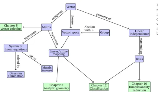
Figure 2.2 A mind map of the concepts introduced in this chapter, along with where they are used in other parts of the book.
Vector
Vector space Matrix
Chapter 5 Vector calculus
Group
System of linear equations
Matrix inverse Gaussian
elimination
Linear/affine mapping
Linear independence
Basis
Chapter 10 Dimensionality
reduction Chapter 12
Classification Chapter 3
Analytic geometry composes
closure
Abelian with+ represents
represents
solvedby
solves
property of
maximalset
resources are Gilbert Strang’s Linear Algebra course at MIT and the Linear Algebra Series by 3Blue1Brown.
Linear algebra plays an important role in machine learning and gen- eral mathematics. The concepts introduced in this chapter are further ex- panded to include the idea of geometry in Chapter 3. In Chapter 5, we will discuss vector calculus, where a principled knowledge of matrix op- erations is essential. In Chapter 10, we will use projections (to be intro- duced in Section 3.8) for dimensionality reduction with principal compo- nent analysis (PCA). In Chapter 9, we will discuss linear regression, where linear algebra plays a central role for solving least-squares problems.
2.1 Systems of Linear Equations
Systems of linear equations play a central part of linear algebra. Many problems can be formulated as systems of linear equations, and linear algebra gives us the tools for solving them.
Example 2.1
A company produces products N1, . . . , Nn for which resources R1, . . . , Rm are required. To produce a unit of product Nj, aij units of resourceRiare needed, wherei= 1, . . . , mandj= 1, . . . , n.
The objective is to find an optimal production plan, i.e., a plan of how many unitsxj of product Nj should be produced if a total ofbi units of resourceRiare available and (ideally) no resources are left over.
If we producex1, . . . , xnunits of the corresponding products, we need
a total of
ai1x1+· · ·+ainxn (2.2) many units of resourceRi. An optimal production plan(x1, . . . , xn)∈Rn, therefore, has to satisfy the following system of equations:
a11x1+· · ·+a1nxn =b1
...
am1x1+· · ·+amnxn=bm
, (2.3)
whereaij ∈Randbi ∈R.
Equation (2.3) is the general form of asystem of linear equations, and
system of linear
equations x1, . . . , xn are the unknownsof this system. Everyn-tuple(x1, . . . , xn) ∈ Rn that satisfies (2.3) is asolutionof the linear equation system.
solution
Example 2.2
The system of linear equations
x1 + x2 + x3 = 3 (1) x1 − x2 + 2x3 = 2 (2)
2x1 + 3x3 = 1 (3)
(2.4) hasno solution:Adding the first two equations yields2x1+3x3= 5, which contradicts the third equation (3).
Let us have a look at the system of linear equations x1 + x2 + x3 = 3 (1) x1 − x2 + 2x3 = 2 (2) x2 + x3 = 2 (3)
. (2.5)
From the first and third equation, it follows thatx1 = 1. From (1)+(2), we get2x1+ 3x3 = 5, i.e.,x3 = 1. From (3), we then get thatx2 = 1. Therefore, (1,1,1) is the only possible and unique solution (verify that (1,1,1)is a solution by plugging in).
As a third example, we consider
x1 + x2 + x3 = 3 (1) x1 − x2 + 2x3 = 2 (2)
2x1 + 3x3 = 5 (3)
. (2.6)
Since (1)+(2)=(3), we can omit the third equation (redundancy). From (1) and (2), we get2x1= 5−3x3and2x2= 1+x3. We definex3=a∈R as a free variable, such that any triplet
5 2−3
2a,1 2 +1
2a, a
, a∈R (2.7)
2.1 Systems of Linear Equations 21
Figure 2.3 The solution space of a system of two linear equations with two variables can be geometrically interpreted as the intersection of two lines. Every linear equation represents a line.
2x1−4x2= 1 4x1+ 4x2= 5
x1
x2
is a solution of the system of linear equations, i.e., we obtain a solution set that containsinfinitely manysolutions.
In general, for a real-valued system of linear equations we obtain either no, exactly one, or infinitely many solutions. Linear regression (Chapter 9) solves a version of Example 2.1 when we cannot solve the system of linear equations.
Remark (Geometric Interpretation of Systems of Linear Equations). In a system of linear equations with two variablesx1, x2, each linear equation defines a line on the x1x2-plane. Since a solution to a system of linear equations must satisfy all equations simultaneously, the solution set is the intersection of these lines. This intersection set can be a line (if the linear equations describe the same line), a point, or empty (when the lines are parallel). An illustration is given in Figure 2.3 for the system
4x1+ 4x2= 5
2x1−4x2= 1 (2.8)
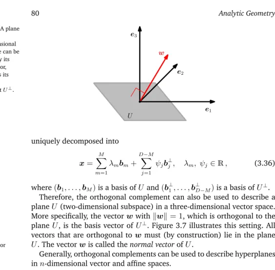
where the solution space is the point(x1, x2) = (1,14). Similarly, for three variables, each linear equation determines a plane in three-dimensional space. When we intersect these planes, i.e., satisfy all linear equations at the same time, we can obtain a solution set that is a plane, a line, a point or empty (when the planes have no common intersection). ♢ For a systematic approach to solving systems of linear equations, we will introduce a useful compact notation. We collect the coefficients aij
into vectors and collect the vectors into matrices. In other words, we write the system from (2.3) in the following form:
a11
... am1
x1+
a12
... am2
x2+· · ·+
a1n
... amn
xn =
b1
... bm
(2.9)
⇐⇒
a11 · · · a1n
... ... am1 · · · amn
x1
... xn
=
b1
... bm
. (2.10)
In the following, we will have a close look at these matrices and de- fine computation rules. We will return to solving linear equations in Sec- tion 2.3.
2.2 Matrices
Matrices play a central role in linear algebra. They can be used to com- pactly represent systems of linear equations, but they also represent linear functions (linear mappings) as we will see later in Section 2.7. Before we discuss some of these interesting topics, let us first define what a matrix is and what kind of operations we can do with matrices. We will see more properties of matrices in Chapter 4.
Definition 2.1(Matrix). Withm, n∈Na real-valued(m, n)matrixAis
matrix
anm·n-tuple of elementsaij,i= 1, . . . , m,j = 1, . . . , n, which is ordered according to a rectangular scheme consisting ofmrows andncolumns:
A=
a11 a12 · · · a1n
a21 a22 · · · a2n
... ... ... am1 am2 · · · amn
, aij ∈R. (2.11)
By convention(1, n)-matrices are calledrowsand(m,1)-matrices are called
row
columns. These special matrices are also calledrow/column vectors.
column row vector column vector Figure 2.4 By stacking its columns, a matrixA can be represented as a long vectora.
re-shape
A∈R4×2 a∈R8
Rm×n is the set of all real-valued(m, n)-matrices.A ∈ Rm×n can be equivalently represented as a ∈ Rmn by stacking all n columns of the matrix into a long vector; see Figure 2.4.
2.2.1 Matrix Addition and Multiplication
The sum of two matricesA∈Rm×n,B ∈Rm×nis defined as the element- wise sum, i.e.,
A+B:=
a11+b11 · · · a1n+b1n
... ...
am1+bm1 · · · amn+bmn
∈Rm×n. (2.12) For matrices A ∈ Rm×n, B ∈ Rn×k, the elementscij of the product
Note the size of the
matrices. C =AB ∈Rm×k are computed as
C =
np.einsum(’il,
lj’, A, B) cij =
n
X
l=1
ailblj, i= 1, . . . , m, j= 1, . . . , k. (2.13)
2.2 Matrices 23
This means, to compute elementcij we multiply the elements of theith There arencolumns inAandnrows in Bso that we can computeailbljfor l= 1, . . . , n.
Commonly, the dot product between two vectorsa,bis denoted bya⊤bor
⟨a,b⟩.
row ofAwith thejth column ofBand sum them up. Later in Section 3.2, we will call this thedot productof the corresponding row and column. In cases, where we need to be explicit that we are performing multiplication, we use the notation A·B to denote multiplication (explicitly showing
“·”).
Remark. Matrices can only be multiplied if their “neighboring” dimensions match. For instance, ann×k-matrixAcan be multiplied with ak×m- matrixB, but only from the left side:
A
|{z}
n×k
B
|{z}
k×m
= C
|{z}
n×m
(2.14) The productBAis not defined ifm̸=nsince the neighboring dimensions
do not match. ♢
Remark. Matrix multiplication isnotdefined as an element-wise operation on matrix elements, i.e.,cij ̸= aijbij (even if the size ofA,B was cho- sen appropriately). This kind of element-wise multiplication often appears in programming languages when we multiply (multi-dimensional) arrays
with each other, and is called aHadamard product. ♢ Hadamard product
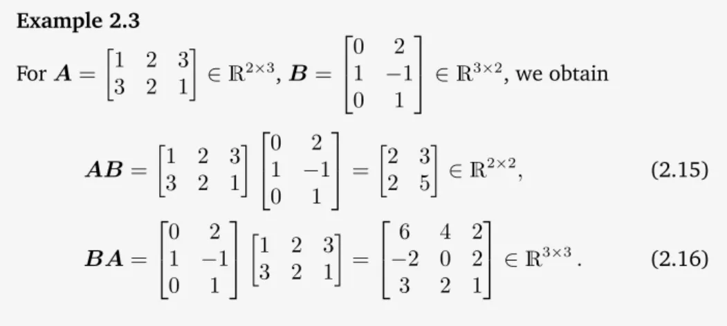
Example 2.3 ForA=
1 2 3 3 2 1
∈R2×3,B =
0 2 1 −1 0 1
∈R3×2, we obtain
AB=
1 2 3 3 2 1
0 2 1 −1 0 1
= 2 3
2 5
∈R2×2, (2.15)
BA=
0 2 1 −1 0 1
1 2 3 3 2 1
=
6 4 2
−2 0 2 3 2 1
∈R3×3. (2.16)
Figure 2.5 Even if both matrix multiplicationsAB andBAare defined, the dimensions of the results can be different.
From this example, we can already see that matrix multiplication is not commutative, i.e.,AB ̸=BA; see also Figure 2.5 for an illustration.
Definition 2.2(Identity Matrix). InRn×n, we define theidentity matrix
identity matrix
In:=
1 0 · · · 0 · · · 0 0 1 · · · 0 · · · 0 ... ... . .. ... ... ...
0 0 · · · 1 · · · 0 ... ... . .. ... ... ...
0 0 · · · 0 · · · 1
∈Rn×n (2.17)
as then×n-matrix containing1on the diagonal and0everywhere else.
Now that we defined matrix multiplication, matrix addition and the identity matrix, let us have a look at some properties of matrices:
associativity
Associativity:
∀A∈Rm×n,B∈Rn×p,C ∈Rp×q : (AB)C =A(BC) (2.18)
distributivity
Distributivity:
∀A,B ∈Rm×n,C,D∈Rn×p: (A+B)C =AC+BC (2.19a) A(C+D) =AC+AD (2.19b) Multiplication with the identity matrix:
∀A∈Rm×n :ImA=AIn =A (2.20) Note thatIm̸=In form̸=n.
2.2.2 Inverse and Transpose
Definition 2.3(Inverse). Consider a square matrixA∈Rn×n. Let matrix
A square matrix possesses the same number of columns and rows.
B ∈ Rn×n have the property that AB = In = BA. B is called the inverseofAand denoted byA−1.
inverse Unfortunately, not every matrix A possesses an inverse A−1. If this inverse does exist, A is called regular/invertible/nonsingular, otherwise
regular invertible nonsingular
singular/noninvertible. When the matrix inverse exists, it is unique. In Sec-
singular noninvertible
tion 2.3, we will discuss a general way to compute the inverse of a matrix by solving a system of linear equations.
Remark(Existence of the Inverse of a2×2-matrix). Consider a matrix A:=
a11 a12
a21 a22
∈R2×2. (2.21)
If we multiplyAwith
A′:=
a22 −a12
−a21 a11
(2.22) we obtain
AA′ =
a11a22−a12a21 0 0 a11a22−a12a21
= (a11a22−a12a21)I. (2.23) Therefore,
A−1= 1 a11a22−a12a21
a22 −a12
−a21 a11
(2.24) if and only ifa11a22−a12a21̸= 0. In Section 4.1, we will see thata11a22−
2.2 Matrices 25 a12a21is the determinant of a2×2-matrix. Furthermore, we can generally use the determinant to check whether a matrix is invertible. ♢ Example 2.4 (Inverse Matrix)
The matrices A=
1 2 1 4 4 5 6 7 7
, B=
−7 −7 6 2 1 −1 4 5 −4
(2.25)
are inverse to each other sinceAB =I =BA.
Definition 2.4(Transpose). ForA ∈ Rm×n the matrixB ∈ Rn×m with
bij =ajiis called thetransposeofA. We writeB=A⊤. transpose The main diagonal (sometimes called
“principal diagonal”,
“primary diagonal”,
“leading diagonal”, or “major diagonal”) of a matrixAis the collection of entries Aijwherei=j.
In general,A⊤can be obtained by writing the columns ofAas the rows ofA⊤. The following are important properties of inverses and transposes:
The scalar case of (2.28) is
1
2+4 =16 ̸=1
2+14.
AA−1=I =A−1A (2.26)
(AB)−1=B−1A−1 (2.27)
(A+B)−1̸=A−1+B−1 (2.28)
(A⊤)⊤ =A (2.29)
(AB)⊤ =B⊤A⊤ (2.30)
(A+B)⊤ =A⊤+B⊤ (2.31)
Definition 2.5 (Symmetric Matrix). A matrix A ∈ Rn×n is symmetricif symmetric matrix
A=A⊤.
Note that only (n, n)-matrices can be symmetric. Generally, we call
(n, n)-matrices alsosquare matrices because they possess the same num- square matrix
ber of rows and columns. Moreover, ifAis invertible, then so isA⊤, and (A−1)⊤ = (A⊤)−1 =:A−⊤.
Remark(Sum and Product of Symmetric Matrices). The sum of symmet- ric matricesA,B ∈ Rn×n is always symmetric. However, although their product is always defined, it is generally not symmetric:
1 0 0 0
1 1 1 1
= 1 1
0 0
. (2.32)
♢
2.2.3 Multiplication by a Scalar
Let us look at what happens to matrices when they are multiplied by a scalarλ ∈ R. Let A ∈ Rm×n andλ ∈ R. ThenλA = K, Kij = λ aij. Practically,λscales each element ofA. Forλ, ψ∈R, the following holds:
associativity
Associativity:
(λψ)C =λ(ψC), C ∈Rm×n
λ(BC) = (λB)C =B(λC) = (BC)λ, B ∈Rm×n,C ∈Rn×k. Note that this allows us to move scalar values around.
(λC)⊤=C⊤λ⊤=C⊤λ=λC⊤sinceλ=λ⊤for allλ∈R.
distributivity
Distributivity:
(λ+ψ)C =λC+ψC, C ∈Rm×n λ(B+C) =λB+λC, B,C ∈Rm×n
Example 2.5 (Distributivity) If we define
C :=
1 2 3 4
, (2.33)
then for anyλ, ψ∈Rwe obtain (λ+ψ)C =
(λ+ψ)1 (λ+ψ)2 (λ+ψ)3 (λ+ψ)4
=
λ+ψ 2λ+ 2ψ 3λ+ 3ψ 4λ+ 4ψ
(2.34a)
=
λ 2λ 3λ 4λ
+
ψ 2ψ 3ψ 4ψ
=λC+ψC. (2.34b)
2.2.4 Compact Representations of Systems of Linear Equations If we consider the system of linear equations
2x1+ 3x2+ 5x3 = 1 4x1−2x2−7x3 = 8 9x1+ 5x2−3x3 = 2
(2.35)
and use the rules for matrix multiplication, we can write this equation system in a more compact form as
2 3 5
4 −2 −7 9 5 −3
x1
x2
x3
=
1 8 2
. (2.36)
Note thatx1 scales the first column,x2 the second one, andx3the third one.
Generally, a system of linear equations can be compactly represented in their matrix form asAx=b; see (2.3), and the productAxis a (linear) combination of the columns ofA. We will discuss linear combinations in more detail in Section 2.5.
2.3 Solving Systems of Linear Equations 27 2.3 Solving Systems of Linear Equations
In (2.3), we introduced the general form of an equation system, i.e., a11x1+· · ·+a1nxn =b1
... am1x1+· · ·+amnxn =bm,
(2.37)
where aij ∈ R and bi ∈ R are known constants and xj are unknowns, i= 1, . . . , m,j= 1, . . . , n. Thus far, we saw that matrices can be used as a compact way of formulating systems of linear equations so that we can writeAx=b, see (2.10). Moreover, we defined basic matrix operations, such as addition and multiplication of matrices. In the following, we will focus on solving systems of linear equations and provide an algorithm for finding the inverse of a matrix.
2.3.1 Particular and General Solution
Before discussing how to generally solve systems of linear equations, let us have a look at an example. Consider the system of equations
1 0 8 −4 0 1 2 12
x1
x2
x3
x4
= 42
8
. (2.38)
The system has two equations and four unknowns. Therefore, in general we would expect infinitely many solutions. This system of equations is in a particularly easy form, where the first two columns consist of a 1 and a 0. Remember that we want to find scalars x1, . . . , x4, such that P4
i=1xici =b, where we definecito be theith column of the matrix and bthe right-hand-side of (2.38). A solution to the problem in (2.38) can be found immediately by taking42times the first column and8times the second column so that
b= 42
8
= 42 1
0
+ 8 0
1
. (2.39)
Therefore, a solution is [42,8,0,0]⊤. This solution is called a particular particular solution
solution or special solution. However, this is not the only solution of this special solution
system of linear equations. To capture all the other solutions, we need to be creative in generating0 in a non-trivial way using the columns of the matrix: Adding0 to our special solution does not change the special solution. To do so, we express the third column using the first two columns (which are of this very simple form)
8 2
= 8 1
0
+ 2 0
1
(2.40)