Modeling, Control and Coordination of Helicopter Systems

Rigorous stability analysis and extensive simulation results demonstrate the effectiveness and robustness of the proposed attitude control. The Q structure allows for automatic scaling of formations according to changes in the overall size of the helicopter team.

Background

In controlling helicopters, an important concern is how to deal with unknown disturbances to the nominal model. The amount of interest in this topic can be attributed to at least two reasons: (1) it is a good platform (and task) to study multi-agent cooperation techniques and (2) there are practical applications for formation control techniques (e.g. in autonomous demining, where a team of demining vehicles must systematically "sweep" through a piece of land).

Outline of the Book

However, constructing the dynamical inversion for a nonaffine system may not be an easy task in general. The second part of the chapter focuses on how the Q structure can be adapted and used for teams where communication is imperfect.

Introduction

General Equations of Motion

• Force Equation
• Moment Equation
• Kinematic Equation
• Navigation Equation

Define L, M, and N as the resultant roll, pitch, and yaw moments along the x, y, z axis, respectively, of the body axis system. In the case of aerodynamic forces and moments, they are typically calculated in the local wind axis system.

Fig. 2.1 Definitions of body axes and hub axes system (Image with courtesy of http://

Modular-Based Modeling

Main Rotor

Elastic modeling of the blade, or even modeling of the blade with finite elements, is only justified if flexibility of the blade is essential. In this case, the vane flap angle is determined by the taper angleˇ0, the longitudinal first harmonic term ˇ1c (positive aft) and the lateral first harmonic termˇ1s (positive toward the forward side).

Fig. 2.2 Block diagram for a general rotorcraft model [97]

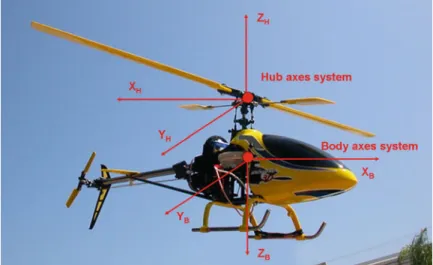
Transformation from Body to Hub

Blade Flapping Dynamics

Without hinge offset, flap spring, and pitch flap coupling, the flap frequency is the same as the rotor frequency. In the first simplification, the rotor is assumed to have no hinge adjustment, no valve spring and no pitch-flap coupling.

Inflow Dynamics

An advantage of using vortex rings is that the effect of vortex rings is non-uniform in terms of relative distance between the rings and the rotor disc. In the ring vortex model, downward velocity due to vortex rings is integrated into the induced velocity calculated by Momentum Theory.

Main Rotor Forces and Moments

This shows that for a hinge displacement or flap spring rotor, the direct hub roll and pitch moments are proportional to the first harmonic pitch of the rotor. As for the resulting roll and pitch moments acting on the vehicle C.G., they are the summation of the direct hub moment and the moments caused by the tilting of the rotor thrust about the body C.G.

Fig. 2.3 Induced velocity variations from Yaggy’s wind-tunnel test [108] and predictions from the ring vortex model: axial and nonaxial flow

Transformation from Hub to Body

For a hingeless or rigid rotor, the direct hub moments can be two to four times greater than the moments from the thrust tilt. Main rotor torque can either be estimated from the rotor power consumption (as will be illustrated in Section.2.4), or from the closed-form expression given as follows. system:.

Tail Rotor

As mentioned earlier, the tail rotor roll and pitch moments are zero due to the staggering configuration. All forces and moments for the tail rotor are transformed back from the hub winding frame to the body frame:.

Propeller

Return to step 3 until the absolute difference (vector norm) between the calculated w and that from the previous calculation is reduced to a desired value. Prediction with Vortex Theory is significantly accurate because it takes into account flow rotation, tip loss, finite blade thickness, and effective blade section curvature due to flow curvature.

Horizontal Tail

In general, lift on the horizontal tail is the dominant force, while the pitch moment is the dominant moment. It may therefore be sufficient to simply calculate the lift and pitch moment from the horizontal tail in certain applications.

Fig. 2.4 Comparison of predictions from Vortex Theory and Momentum-Blade Element Theory with experiment from [37]

Wing

Vertical Tail

Fuselage

Aerodynamic Interference

Rotor Rotational Degree of Freedom

Flight Control System

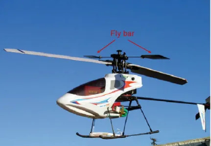
The flybar deserves an in-depth discussion, as it is a common feature found in the 2-blade wobble rotor configuration. One advantage of the Bell-Hiller rod is that it introduces flexibility to adjust the delay to the cyclic controls, since the rotor blades are now controlled by both the pitch of the fly rod and a portion of cyclic controls.

Fig. 2.6 Teetering rotor configuration with a fly bar for a model helicopter

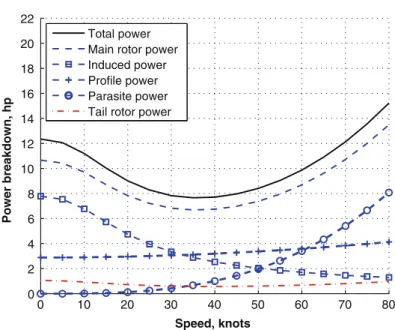
Helicopter Performance Prediction

Normally, the tail rotor power is about 10% of the main rotor power in hover and low speed flight. A simple way to calculate tail rotor power is to use 10% of main rotor power for hover and 5% for high speed.

Table 2.1 RMAX general

Conclusion

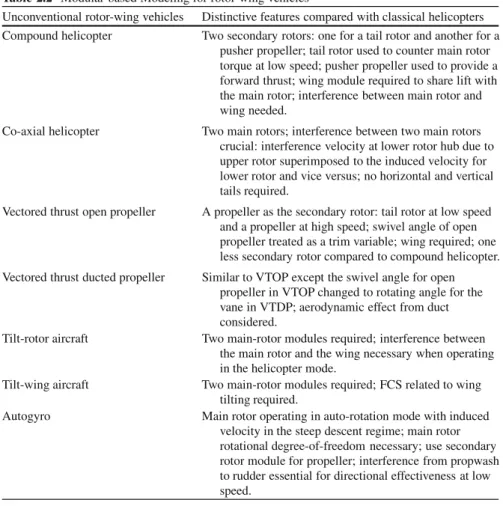
Tilt-rotor aircraft Two main rotor modules required; interference between the main rotor and wing required when operating in helicopter mode. Autogyro Main rotor operates in induced velocity autorotation mode in the steep descent regime; degree of rotational freedom of the main rotor necessary; use secondary rotor module for propeller; interference from propwash to rudder essential for low speed directional effectiveness.

Table 2.2 Modular-based Modeling for rotor-wing vehicles

Introduction

Trim

The singularity of the Jacobian matrix can occur in extreme flight conditions such as Vne flight (never overspeed). In some truncation conditions, collective step 0 is not one of the truncation variables as it is set by a default value.

Linearization

However, there are gravitational and inertial terms in the matrix, which can be obtained accurately by an analytical study of the equations of motion. The linearization of the mathematical model in (3.16) can be performed by expanding the nonlinear function into a Taylor series around the operating point and neglecting the higher-order terms of the expansion [74].

Table 3.2 Symbols and subscripts of helicopter model in hover

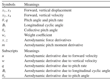
Description of Stability and Control Derivatives

In forward flight, a positive increase in angle of attack causes the rotor to tilt backward, creating nose-up torque to further increase the angle of attack. Another interesting interpretation of the above equation is that when the hull tilts with a constant pitch velocity qH, the time difference between the hull and the rotor is ˝16 s.

Yamaha R50 Helicopter at Hover

An approximation can be made by further assuming that the HIV dynamics are independent of the residual dynamics. From the figure, it can be seen that the differences in eigenvalues ​​from both approximate dynamics and full dynamics are imperceptible.

Fig. 3.1 Eigenvalue plot for Yamaha R50 helicopter at hover

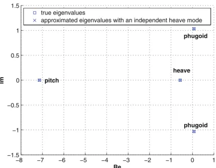
Copterworks AF25B Helicopter in Forward Flight

Far away from the imaginary axis in the left half of the complex plane is the pitch/pitch oscillation mode. In particular, the phugoid mode is closest to the imaginary axis, indicating a minimum stability limit.

Fig. 3.4 AF25B radio control helicopter from Copterworks(Courtesy of Copterworks Inc.)

Conclusion

Introduction

60 4 Height control of helicopters with unknown dynamics In [41], model-based control was applied to the non-linear motion control of a helicopter. How to deal with model uncertainties and distortions is one of the important issues in helicopter control.

Problem Formulation and Preliminaries

Based on Assumption 4.4, the following lemma is given to prove the existence of an implicit desired function, which will be used in the design of the LV controller. The combination of the Implicit Function Theorem, the Mean Value Theorem, and the NN is key to solving the control problem for generalized non-affine helicopter systems described by (4.1).

Function Approximation with Neural Networks

Function Approximation with RBFNN

Function Approximation with MNN

66 4 Height control of helicopters with unknown dynamics In general, ideal weights are unknown and must be estimated when designing the controls. 30] Using fmnn DOWTS.VOTZ/ to approximate the ideal function f .Z/, its approximation error can be expressed as.

Adaptive NN Control Design

Full State Feedback Control

As a result, we can conclude that the states of the internal dynamics will converge to the compact set. It follows that by properly tuning the parameters, the guaranteed upper limit for the steady-state tracking error can be reduced.

Output Feedback Control

80 4 Altitude Control of Helicopters with Unknown Dynamics We are ready to summarize our results for the output feedback case under the following statement. For this case we want to show that, due to z being bounded, the function Kin (4.87) is also bounded, for which (4.83) can be expressed in the form of (4.9), convenient for establishing SGUUB property.

Simulation Study

Linear Models

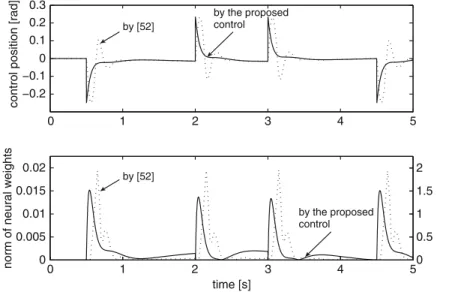
To compare our controller with that of [54], we consider tracking the height along a desired trajectory hd.t /defined by. To compare our controller with that of [38], we consider the tracking of the pitch angle according to a desired trajectoryd.t /defined at.

Fig. 4.1 Comparison of altitude tracking performance between the proposed controller and that of [54]

Nonlinear Model

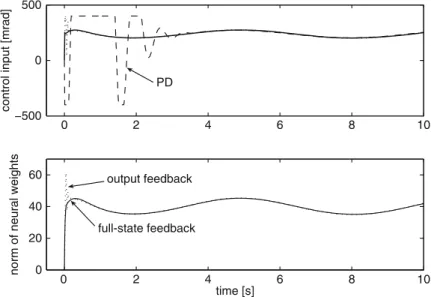
Figure 4.4 shows that the tracking performance of our controller is comparable to that of [38] for the height tracking task. Figure 4.8 shows that the rotor speed and total pitch angle for full-state control and LV output feedback are limited.

Fig. 4.4 Comparison of pitch tracking performance between the proposed control and that of [38]

Conclusion

Introduction

94 5 Pitch and yaw control of helicopters with Uncertain Dynamics function neural network (RBFNN) is used in control design and stability analysis. Based on Lyapunov synthesis, the proposed adaptive NN control ensures that both the height and the yaw angle track the given bounded reference signals to a small neighborhood of zero and guarantees the semi-globally uniform ultimate bound (SGUUB) of all the closed loops. signals at the same time.

Problem Formulation and Preliminaries

Therefore, there are always some positive constantsb11 such that 0b11 is jb11.qP3/j during the vertical flight mode. 96 5 Altitude and Swing of Helicopters with Uncertain Dynamics The following technical lemma is needed in subsequent control design and stability analysis.

Control Design

RBFNN-Based Control

By using WO1 to approximate W1, the error between the actual and the ideal RBFNNs can be expressed as. Using WO2 to approximate W2, the error between the actual and the ideal RBFNNs can be expressed as.

MNN-Based Control

To analyze the closed-loop stability for subsystem q2, consider the following candidate Lyapunov function. According to Assumptions 5.1-5.6, the general closed-loop neural control system is SGUUB in the sense that all signals in the closed-loop system are bounded and the tracking errors and weights converge in the following regions.

Simulation Study

Internal Dynamics Stability Analysis

It then follows that the internal dynamics of the helicopter system in (5.1) has a stable behavior. From Fig.5.1, we can observe that the main rotor angular velocity qP3 converges to the nominal value 124:63 rad/s for different initial conditions ranging from 40rad/s to 150 rad/s, which includes the typical operating values ​​more than adequately.

Performance Comparison Results Between

It can be observed from Figures 5.2 and 5.3 that due to the existence of model uncertainty, both altitude tracking and yaw angle tracking using model-based control have some deviations from the desired trajectories for the whole period. This means that model-based control is highly dependent on model accuracy and cannot deal well with uncertainties.

Fig. 5.2 Altitude tracking performance in the presence of model uncertainties

Conclusion

Introduction

Problem Formulation

To facilitate control system design, we assume that all states of the helicopter attitude dynamics (6.13) are measurable. To improve the robustness of the attitude control, the robust attitude control of helicopters using neural networks was designed in section 6.4.

Model-Based Attitude Control for Nominal Plant

In the following sections, we start from the model-based attitude control for a nominal plant in Sect.6.3 with the free of the uncertaintyF1.x1; x2/and external disturbance D.x1; x2; t / of the system (6.13). Considering the nominal attitude dynamics of the helicopter system (6.13), the model-based control law is formulated according to (6.29).

Robust Attitude Control of Helicopters with Uncertainties

0,K2 D K2T > 0inK3 D K3T > 0so that the entire closed-loop control system is semi-globally stable in the sense that all closed-loop signals z1, z2, z3inQ are bounded. When kz3k< "3, we can also conclude that all signals of the closed-loop system are bounded based on Lemma 6.1 if only the appropriate design parameters K1 and K2 are chosen with respect to the bounded F2.x3/.

Approximation-Based Attitude Control of Helicopters

Considering the stability of the error signals Q1 and Q2, the candidate for the extended Lyapunov function can be written as In order to achieve stability for 'Q error signals, a candidate for the extended Lyapunov function can be chosen.

Simulation Results

Model-Based Attitude Control

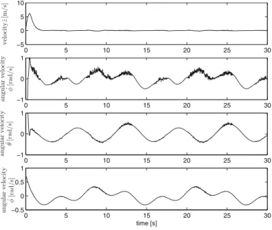
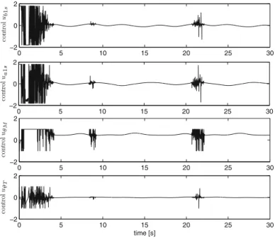
From Fig.6.2 we know that the velocity along z-axis and angular velocity under the model-based control converge to a small neighborhood of the origin. Figure 6.3 shows that the command control signals are saturated within the limits of the actuators.

Fig. 6.2 Velocity along z axis and angular velocity signals using the model-based control

Robust Attitude Control

From Figure 6-5, the velocity along the z-axis and the angular velocity with the uncertainties and perturbations can converge to a compact set.

Approximation-Based Attitude Control

Figure 6.6 shows that the command control signals are saturated within the limits of the actuators. From Fig.6.8, it can be observed that the line velocity along the z-axis and the angular velocity of the glide converge to a small quarter of the origin.

Fig. 6.6 The command control signals using the robust attitude control

Conclusion

Introduction

The main purpose of the kinematic controller is to generate a desired reference plan and/or trajectory for each helicopter in the team, which is then passed to the lower level helicopter controllers who take into account the dynamics of each helicopter. The chapter begins by exploring the use of the Q-structure for formation control where perfect communication is present between all members of the team.

Q-Structures and Formations

• Assumptions
• Division of Information Flow
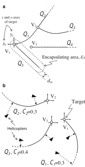
• Elements of the Q-structure
• Properties of the Q-structure

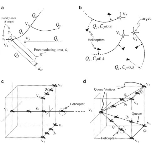
The main difference between the proposed approach and other approaches (such as [17, 20]) is the use of the Q structure. Typical graphic representations of formations rely on precise placement of each helicopter to achieve the final appearance of the formation.

Fig. 7.2 Examples of queues, and formation vertices (circles), where x t and y t are the axes of the coordinate frame of the target centered at V 1

Q-Structure with Perfect Communication

• Changing Queues
• Potential Trench Functions
• Helicopter Behaviors
• Simulation Experiments

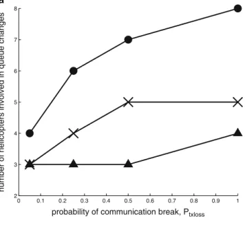
Five images of nine helicopters entering a wedge formation during the simulation are shown in Figure 7.11. For Iloss D 0:50 with communication disruptions for 5% of the time, the queue state of the nine helicopters in the team is shown in Figure 7.21.

Fig. 7.5 Examples of queues, and formation vertices (circles), where x t

Q-Structure with Imperfect Communication

Determination of Target on Queue

It works through the helicopters within communication range ofri which should also be considered on the same queue asri. The target changes in response to the information it has from other helicopters within communication range and that are in the same line.

Fig. 7.22 Effect of different degrees of communication breakdown on the formation. Circle

Navigation of Helicopters to Positions in Formations

To show that the remaining critical points of the system, i.e., qc, are unstable equilibrium points, consider the following. For a helicopter, other helicopters can be treated as obstacles, and the equilibrium points are a direct result of the relative positions.

Simulation Studies

Conclusion

Introduction

Problem Formulation

Helicopter Dynamics

Formation Control of Helicopters

Control with Full Information

Control with Partial Information

Simulation Study

Conclusion