This text is intended for students interested in the design of classic and new IC motor control systems. We would like to express our gratitude to the many colleagues and students who have reported errors and omissions in the first edition of this text.
Notation
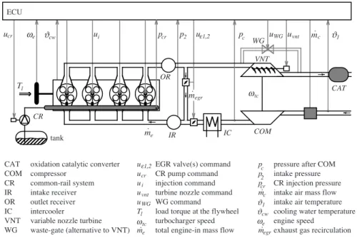
It also contains some general notes on electronic engine management systems and introduces the most common control problems encountered in spark ignition (Otto or gasoline) and compression ignition (Diesel) engine systems. In a turbocharged engine system, the four most important locations are designated by the indices 1 for "before compressor", 2 for "after compressor", 3 for "after engine" and 4 for "after turbine".
Control Systems for IC Engines
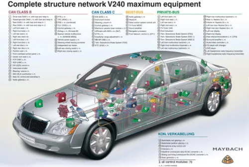
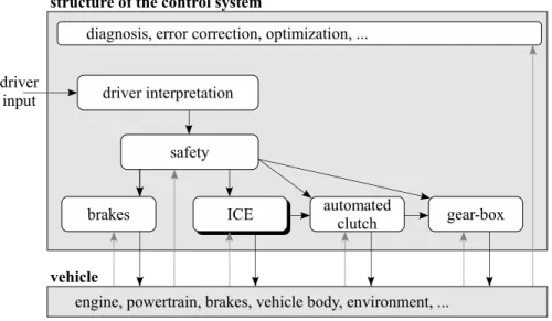
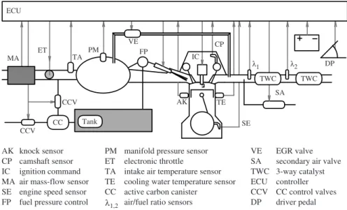
In this text, only the "ICE" (i.e., the engine and the corresponding hardware and software necessary to control the engine) will be discussed. Typically, an electronic engine control unit (ECU) includes standard microcontroller hardware (process interfaces, RAM/ROM, CPU, etc.) and at least one additional piece of hardware, often designated as a timing processing unit (TPU), see Fig.
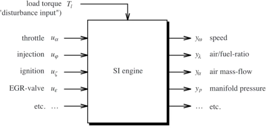
Overview of SI Engine Control Problems
The air/fuel ratio feedback control system compensates for the inevitable errors in the forward motion circuit. While it guarantees that the average value of the air/fuel ratio is at the stoichiometric level, it cannot prevent transient excursions in the air/fuel ratio.
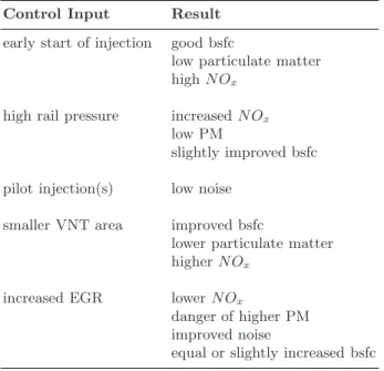
Overview of Control Problems in CI Engines
EGR flow greatly affects the flow of air mass through the intake and exhaust manifolds. These filters allow an engine calibration in high PM/low N compensation oxide.
Structure of the Text
This allows the engine to be calibrated at the high-efficiency/low-PM boundary of the trade-off curve (see Fig. 1.11, early injection angle). A good overview of the first developments in the field of MVM of SI engine systems can be found in [167].
Introduction
Discrete event models (DEM), i.e. COM, which explicitly takes into account the reciprocating behavior of the motor. 3 In MVM, the finite sweep volume of the engine can be seen as one that is distributed over an infinite number of infinitely small cylinders.
Cause and Effect Diagrams
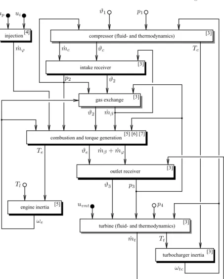
In the cause and effect diagram, the named reservoirs appear as blocks with black shading. In the intake and exhaust manifolds, for example, not only masses but thermal (internal) energy are important.
Air System
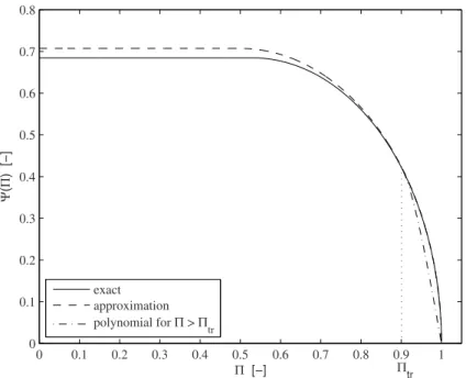
Substituting (2.5) and (2.6) into (2.3) and (2.4), the following two differential equations for the plane variables pressure and temperature (which are the only measurable quantities) are obtained after some simple algebraic manipulations. The power absorbed by the compressor is the isentropic power Pc,s (i.e. the power required by a "perfect" compressor to compress the mass flow of gas from its input to its output pressure level), divided by the isentropic efficiencyηc which takes taking into account all the inevitable deterioration in the actual technical compressor realization. 2.39) Since the compressor speed is level variable (i.e. an available output of a store), the torque absorbed by the compressor can be easily found from equation (2.39). 2.40) Similarly, the temperature increase due to the compression is formulated as an isentropic (unavoidable) part and an additional increase due to technical imperfections in the compressor realization. 2.41) Note that in equation (2.41) adiabatic conditions have been assumed, i.e. heat losses through the compressor walls and in the compressor outlet will have lowered the gas temperature before it enters the intercooler or the intake manifold.
Fuel System
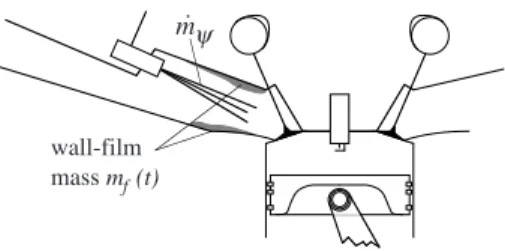
One of the most important dynamic effects on the fuel path is due to the wetting of the walls. The kinematic viscosityν depends on the temperature of the liquid and can also be taken from the tables. To calculate the Reynolds number, the velocity of the droplets must be calculated.
Then, due to the geometry of the intake runner, some drops will hit the manifold walls. By assuming δth ≪ dF, this identification results in a relevant area AF for the evaporation of the wall film of. This gas fraction carries the air/fuel ratio of the current cycle forward to the next.
Mechanical System
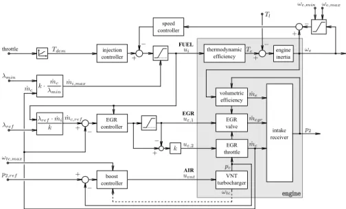
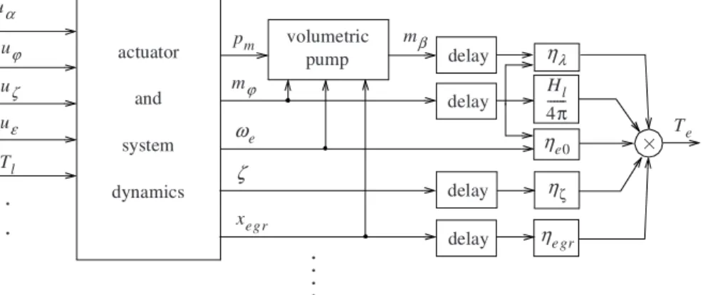
The factor eλ(λ) models the influence of the changing air/fuel ratio on the thermodynamic efficiency. The form of this reduction, primarily an approximation, is independent of the operating point and of the engine type [70]. The factor eegr(xegr) models the influence of the changing burnt gas fraction on the thermodynamic efficiency.
The numerator is proportional to a fictitious pneumatic energy stored in the manifold, while the numerator is proportional to the kinetic energy of the engine flywheel. The stiffness of the spring and the damping coefficient determine the characteristics of the axis connecting the two inertias. 35 In a well-dimensioned dynamic test bench configuration, the inertia of the motor is several times smaller than that of the test bench brakes.
Thermal Systems
Disregarding these deviations, a qualitative approach would be to assume that the engine-off temperature is an affine function of the engine's mechanical power. The radiation terms are proportional to the difference in the fourth power of the temperatures. The numerical values of the parameters are adapted to the standard conditions of the exhaust manifold of the SI engine.
In this section, a simple model of the motor thermal behavior is first introduced, which can be used, for example, in combination with the. Influence of the cylinder wall temperature on the heat flow from the cylinder to the wall (as average pressure [bar]), for different loads. Assuming that the velocities (control inputs) change slowly compared to the magnitude of the time delays, the variable τi→j can be approximated by. 2.174).
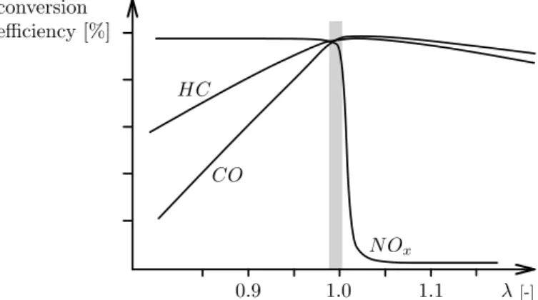
Pollutant Formation
This dependence of the reaction rate on the gas temperature is the main reason for the high concentrations of NO in the exhaust gases. Global air/fuel ratios do not represent the local air/fuel ratio at which the actual combustion process takes place. The inhomogeneity of the air/fuel mixture is also the main cause of the formation of solid particles.
Instead, an approximation of the following form can be used to estimate the concentrations of the engine outN Emissions. As mentioned in the introduction to this section, this is the best that can be expected from COM of the contaminant formation. Note that (2.186) quantifies the concentration of the pollutants in the exhaust gas, i.e. the number of NO molecules relative to the total number of parts in the exhaust gas (usually mol/mol).
Pollutant Abatement Systems
Other applications are the optimization of the catalyst system and the development of improved controls. The free volume (i.e. the volume accessible to the gas) per length of the washcoat is given by 4db·εW·dW. The dynamics of the gas concentrations in the channel can be omitted and thus the gas concentrations are calculated quasi-statically.
Finally, the mass balances of the adsorbed species on the catalyst surface are calculated as follows. The capacity of the oxygen storage can be estimated from the emission measurement data and a relative oxygen content can be calculated. The model can reproduce the dynamic behavior of the catalytic converter during a driving cycle.
Pollution Abatement Systems for Diesel Engines
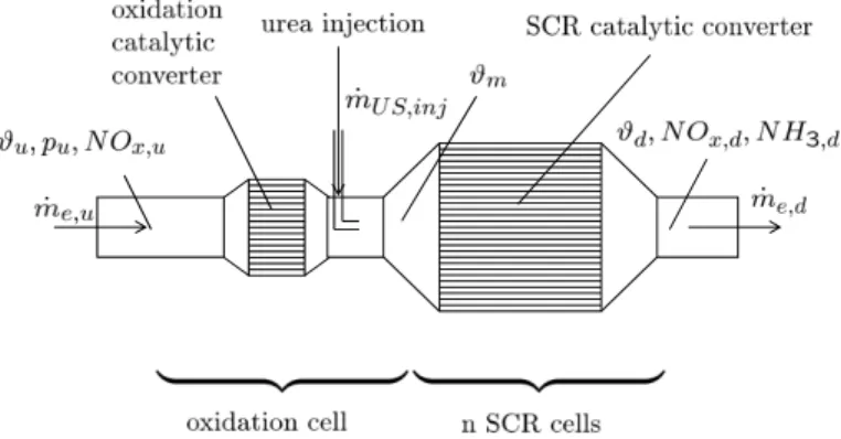
Adsorption and desorption of ammonia on the surface of the catalytic converter (where∗ denotes an adsorbed species). It is useful to mount an oxidation catalytic converter before the SCR catalyst. Complete SCR system consisting of the oxidation catalytic converter, the urea injection device and the SCR catalytic converter.
Adsorption and desorption of ammonia on the surface of the catalyst is described using (2.230). The oxidation of the ammonia adsorbed on the surface of the catalyst is modeled using (2.233). The oxidation of ammonia on the surface of the catalyst has also been taken into account.
Introduction to DEM
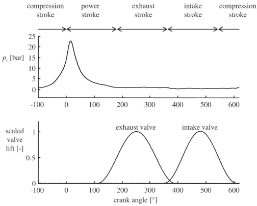
In the remaining portions of the two revolutions, the engine rotates due to the inertia of the flywheel. The primary task of the ECU is to guarantee the injection of the correct amount of fuel into the manifold and the ignition of the mixture in the cylinder at the desired crank angle position with sufficient energy. The lift curves of the intake and exhaust valves of an engine are assumed to be constant in the crank angle domain (this is obviously not the case with variable valve timing).
In addition, new values for the duration of the injection duration (as well as for the ignition time) are sent to the time processing unit (TPU). To summarize these considerations, the time delay between the start of the computation (injection event update) and the injection start event can be approximated by . τc)−e)=τcalculation+1. At point a, the measurements of the engine variables necessary for determining the ignition timing are activated by the ECU.
The Most Important DEM in Engine Systems
Again, assuming that the fuel dynamics for each cylinder are first order, the system depicted in Fig. In the following, a model of the backflow dynamics first introduced in [54] is presented. The simulation combines the discrete-event model with a continuous-time model of the sensor dynamics.
Therefore, formulating a mass balance of both the fresh charge and the burnt gases present in the cylinder after the intake valve is closed yields the following equation for the air/fuel ratio λ(k) of the engine displacement. A very rough estimate would be a value for mrg of 5% of the total mass at full load in the cylinder. In this section a DEM of the effects taking place in the exhaust system is presented.
DEM Based on Cylinder Pressure Information
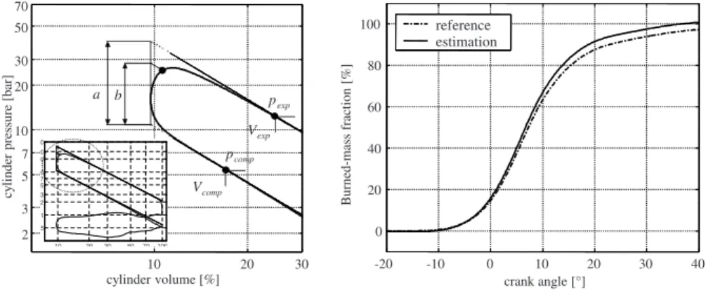
A typical application for the method introduced in the last section is the estimation of the 50% burned mass position. A computationally more demanding use of the pressure trace, which is based on physical first principles, is the estimation of the fresh air, fuel and burned gas mass in the cylinder. The variable mbg=mrg+megr is the total mass of burned gas, i.e. the sum of the residual gas and the externally recirculated exhaust gas.
Once the total mass is known, the amount of gas burned can be estimated if the mass of aspirated mixture is estimated with one of the methods presented in both sections. For the relevant operating range of a six-cylinder 3.2-liter SI engine, the pressure difference as a function of combustion energy is depicted in fig. These observations lead to the following parameterization of the pressure difference as a function of engine speed and heat release center.