Some examples of cellular automata used for modeling purposes include: lattice gas cellular automata [18]. In this work, we compare the predictive power of standard cellular automata with a specific class of CA, called cellular automata networks (CAN), using a large amount of climate data from the National Center for Environmental Prediction (NCEP)/National Center for Atmospheric Research. (NCAR) Reanalysis 1 dataset [5]. Previous work on networks of cellular automata and modeling climate data as complex networks, discussed in Chapter 2, suggests that CAN can be used to model climate data.
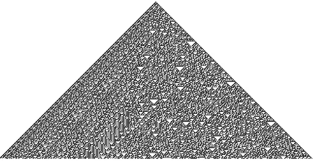
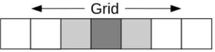
The combined ideas from all these sections support our goal of showing how cellular automata networks can be used to model climate data as a complex network. Cellular Automata were first described by John von Neumann in the late 1940s in his work on creating an abstract universal constructor. Briefly, a cellular automata consists of a grid (or lattice), a neighborhood and a transition function.
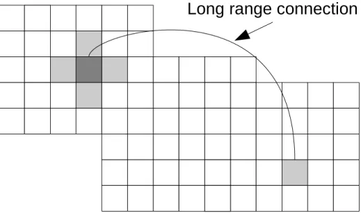
The grid on which cell automatons run can also be modeled as a network where each cell is connected to its cell. Standard cellular automata can be thought of as networks where each cell in the automaton is a vertex. When a cellular automata network is used, as described in [21], the resulting network behaves like a complex network (or small-world network).
Cellular automata networks are an extension of cellular automata that allow for non-local (or long-distance) connections to other cells.
EXPERIMENT DESIGN
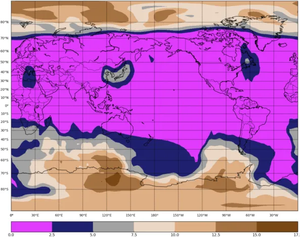
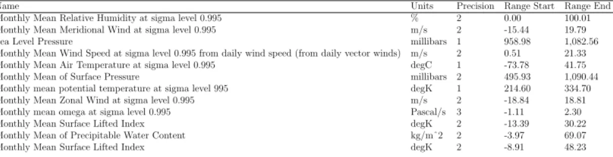
To reduce the computational effort, we will use the monthly averages of the twelve surface-level variables included in the “NCEP/NCAR Reanalysis Monthly Means and Other Derived Variables” subset. The dataset is distributed in the NetCFDF4 file format with a single file for each of the 12 variables. Relative humidity: the ratio of the partial pressure of water vapor in the mixture to the saturated vapor pressure of water at a given temperature.
At each cell location there are 802 measurements (once per month from January 1948 to October 2014) for each of the 12 surface-level variables in the dataset, for a total of measurements. In this description of the data set, a horizontal cross section at a point along the vertical axis would be a description of the entire map at that point in the time series. The objective of the first experiment is to determine a baseline result that we hope to be able to beat with a mobile automaton implementation.
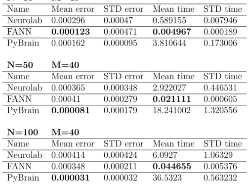
Python2 bindings of the FANN library[7] are used to train all neural networks in our experiments. In this case, each cell in the grid will have an individual neural network trained on the first half of the time series data from the variables in its Von Neumann neighborhood. Similar to the previous experiment, the neural networks are tested on the second half of the data, and the mean absolute error (MAE) and mean square error (MSE) metrics are recorded for each variable.
The cellular automaton functionality of the model is tested by simulating climate variables, starting with baseline data. As expected, the predicted values from this model are not representative of the data since the linear regression method cannot model the seasonal component of the data. You can see from this plot that the predictions generally match the shape of the input data, but do not model any anomalies in the data.
The strong fit to the first half of the data compared to the loose fit to the second half suggests that the Cascade Correlation training method is adapting the neural networks to the data seen. The first part of the experiment tests the neural networks on the single variable air temperature. In the second part of the experiment, the mobile automaton part of the model was used.
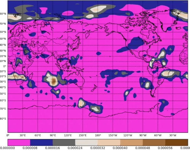
Air temperature in the northern US, Canada and northern Asia seems to be difficult to predict compared to the rest of the world. As mentioned in the experimental design in Section 3.5, the locations for the long-range links in the cellular automaton network were randomly selected from a list of the top 200 highly correlated cells.
CONCLUSION
More experiments could be done immediately with the same and different data sets to support our primary conclusion that cellular automata networks are better suited than cellular automata to model complex network-based problems. More work could also be done in designing experiments that compare cellular automata networks with cellular automata where the effectiveness of the transition function is known in advance. This would allow stronger conclusions to be drawn about the effectiveness of the two different techniques.
More experiments using cellular automata networks to model complex networks should be conducted to explore the extent of cellular automata performance in these applications. This work only compared cellular automata networks with cellular automata, but future work could compare the performance of cellular automata networks with other simulation techniques. To set up cellular automata network tests, we needed a library for fast and easy training of neural networks from Python.
The training input was floating point random numbers in the interval and the output was the sum of the inputs. Considering that the FANN library is still an active project, its extremely fast training time compared to the other two libraries, and the good results from training on benchmark data, we will use the FANN library for mobile automaton experiments. . Resources provided by the Mississippi Center for Supercomputing Research (MCSR) were used to run the largest full cellular automaton experiments for this study.
All the supporting libraries and their dependencies used had to be built from source in the home directory. Run the client.py script for each longitude cell in the current row, parallelize this process using all the processors available for the current node3. 3runner.py with latitudeLA will spawn an X number of processes each running 144/X experiments for the given LA, where X is the number of processors available on the given node.
To keep the experiment code as separated from the process as possible, we created the runner.py script to handle the parallelization in the node. To run a batch experiment, first ran the queueAll.sh script from rows 0 to 39 (“./queueAll.sh 0 39”) and then ran “touch runNext” to run the watchdog. py script to execute the next set of commands after the current set is completed. The nodes running the client.py script are not connected to external networks, making it impossible for them to report their results directly to a database.
Instead of reporting results automatically, each experiment writes its results to a file and at the end of a macro experiment an updateDB.py script is called which parses all output files and updates a Redis database running on our workstation . in the Computer Science Department. An example call to client.py for certain latitude and longitude cell indexes and usage for the script are as follows:


![Figure 4.2: Linear regression model for Air Temperature on cell [23,108].](https://thumb-ap.123doks.com/thumbv2/123dok/10461891.0/30.918.208.770.157.455/figure-linear-regression-model-for-air-temperature-cell.webp)