Introduction
Optimal data-dependent regret through 𝐻 ∞ control
This is a 𝐻∞ condition; its interpretation ensures that the cost incurred by the controller𝜋 in the synthetic system is less than the energy of the synthetic disturbance ˆ𝑤. One particularly interesting choice of complexity measure we consider is 𝐶(𝑤) = 𝐽(𝜋 . 0, 𝑤); in this case, the limit (1.1) can be rearranged to obtain the competitive ratio limit, which is the worst possible ratio between the costs incurred by the causal policy𝜋 and the costs incurred by the optimal non-causal policy𝜋.
Preliminaries
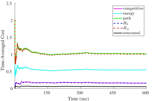
In Theorem 5 we show that the time-averaged expected cost of the noncausal optimal controller converges to . We see in Figure 6.8 that the 𝐻∞ controller exactly matches the performance of the non-causal optimal controller, while the competitive one and 𝐻.
The Optimal Noncausal Controller
An operator-theoretic model of the optimal noncausal controller
Recall that the cost incurred by a controller which selects the control sequence 𝑢 in response to the disturbance sequence𝑤 is . The first term clearly does not depend on 𝑢, whereas the second term can be set to zero by setting .
A factorization of the offline optimal cost
A state-space model of the optimal noncausal controller
We emphasize that the optimal offline control actions are defined with respect to the actual realizations𝑤. 𝑤𝑇; the optimal offline control actions are the optimal actions afterwards, with full knowledge of the realization𝑤. In other words, the optimal offline control action in time step𝑡is the sum of the𝐻.
- the existence of the controller, which is unfortunately limited by the length of the drive disturbance path and measurement disturbance. The 𝐻∞-optimal controller has 𝛾 = 1.00, so the cost incurred by the 𝐻∞ controller is at most the disturbance energy.
Regret-Optimal Full-Information Control
Competitive Control
Plugging these parameters into Theorem 17 immediately yields necessary and sufficient conditions for the existence of a causal competitive-suboptimal controller at level𝛾, along with a state-space model for the controller, if it exists. The operatorΔ−1(𝑧)𝐺(𝑧) is given by. 3.9) We emphasize that the system whose frequency domain dynamics is given by (3.8) is driven by 𝑤b𝑡+. We interpret 𝐼+𝐹 𝐹⊤as the covariance matrix of an appropriately defined random variable and use the Kalman filter to obtain a state-space model for Δ.
Given a state space model for 𝐹, a Kalman filter can be used to construct a state space model for the causal matrix Δ such that 𝑦= Δ𝑒 where 𝑒 is a random variable with zero mean such that E[𝑒 𝑒⊤] = 𝐼; this is the so-called "whitening" property of the Kalman filter. Now that we have state space models for 𝐹inΔ, we can construct a state space model for the entire system (3.12).
Energy-Optimal Control
We immediately obtain the factorization (3.17), where we define 3.19) Recall that the energy suboptimal controller at level 𝛾 is the 𝐻∞ suboptimal controller at level 1 in the system (3.18). Furthermore, one can check that the stabilizability of (𝐴, 𝐵𝑢) implies the stabilizability of (b𝐴,𝐵b𝑢), and similarly the observability of (𝐴, 𝐿) implies the unit circle observability of (𝐴,b 𝑢b). We have shown that the energy suboptimal controller at level 𝛾 in the system {𝐴, 𝐵𝑢, 𝐵𝑤, 𝐿} is the 𝐻∞ suboptimal controller at level 1 in the system {b𝐴,𝐵b𝑢,𝐵},b𝐴,𝐵b𝑢,𝐵} is.
It is easy to find out the strictly causal energy suboptimal controller analogously. Recall that the synthetic perturbation𝑤 is given by 𝑤b(𝑧) = Δ2(𝑧)𝑤(𝑧); from (3.19) it immediately follows that there is a state space model for 𝑤bis.
Pathlength-Optimal Control
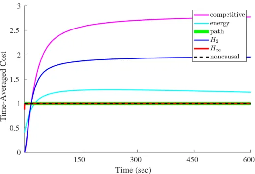
In this section, we describe a causal controller 𝜋 whose regret is bounded by the path length of the row perturbation and the energy of the measurement perturbation. The competition controller has 𝛾 =2.14; in other words, the competitive ratio of the competition controller is 4.58. We see that the energy-optimal controller incurs costs that are approximately halfway between those of the.
In this section, we study the behavior of the competitive controller in the classical nonlinear inverted pendulum system. Moreover, when the disturbance is stochastic, the competitive controller can almost match the performance of the𝐻.
Regret-Optimal Measurement-Feedback Control
Non-existence results
In the measurement-feedback setting, the controller is unable to directly sense, and must therefore set 𝑢 =0 at all times. In the measurement-feedback setting, the controller is unable to directly sense 𝑤 and 𝑣, and must therefore set 𝑢 = 0 at all times. In this section, we establish that in unstable systems there is no controller whose regret is bounded by the energy of the driving disturbance and the path length of the measuring disturbance.
In the measurement-feedback setting, the controller cannot directly observe 𝑤 and 𝑣, so it must always set 𝑢 = 0. The only setting where this "null controller" can regret being limited by the energy of the drive disturbance and the path length of the measurement disturbance is when the system is stable.
Regret bounded by the joint energy of 𝑤 and 𝑣
𝐾bitself described the form of a transfer operator in (4.1); it is the transfer operator with Youla parameter𝑄b=𝛾−1𝑄in the system. It is now clear that a controller 𝐾 satisfying (4.6) exists if and only if there exists a controller 𝐾in the system (4.9) such that ∥𝑇. 2 is stable and thus Δ−1(𝑧) is causal and bounded since its poles are strictly contained in the unit circle.
Regret bounded by the pathlength of 𝑤 and the energy of 𝑣
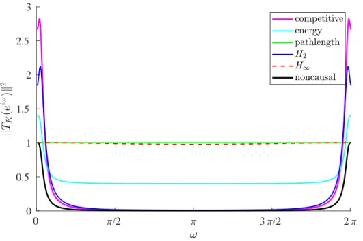
The energy-optimal controller has𝛾 =0.63; in other words, the regret of the energy-optimal controller versus the optimal non-causal controller is bounded by 0.4 times the energy of the perturbation. We see that the frequency response of the 𝐻∞ controller peaks at 𝜔 = 0, where it matches the frequency response of the optimal non-causal controller; all other causal controllers have a higher peak frequency response. In other words, the energy-optimal controller minimizes the gap between its own frequency response and the frequency response of the optimal non-causal controller.
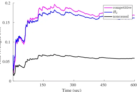
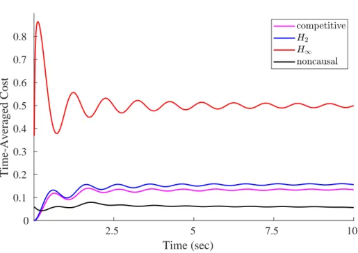
In Figure 6.3, we plot the costs of just the competing and 𝐻2 controllers to better illustrate how well the competing controller can approximate the performance of the 𝐻. The frequency responses in Figure 6.1 predict that the competing controller will perform the worst, while the path length optimal and 𝐻∞ controllers will match the performance of the optimal non-causal controller; this prediction is confirmed in Figure 6.4.
Connections to Online Learning
Approximation of the competitive controller by DAC policies
We prove that we can find a DAC policy which generates a sequence of states and control actions that closely follows the sequence of states and control actions generated by the optimal competing policy by taking the history and weights appropriately. We recall that 𝐴b+𝐵b𝐾bis stable; this matrix is upper-triangular block, and the matrix in block (1, 1) is 𝐴+𝐵𝐾b. We now describe a DAC policy ˜𝜋𝑐 which approximates 𝜋𝑐; recall that each DAC policy is parameterized by a stabilizing controller and a set of weights 𝐻.
We combined the pieces to limit the difference in costs caused by competing policies and our DAC approximation at each time step.
Best of both worlds: sublinear policy regret implies approximate
The goal of the controller is to stabilize the object by keeping (𝑥 ,𝑥¤) as close to (0,0) as possible, while using little energy. The path length optimal controller has𝛾 =934.99; in other words, the regret of the path length optimal controller versus the optimal non-causal controller is bounded by 8.74×10⁵ times the path length of the disturbance. Intuitively, this is because the competitive controller is constrained to maintain a frequency response within a factor of 4.58 of the frequency response of the optimal non-causal controller, so it has more leeway at frequencies near 𝜔 = 0 and𝜔 = 2𝜋, where the optimal non-causal controller also has a high frequency response.
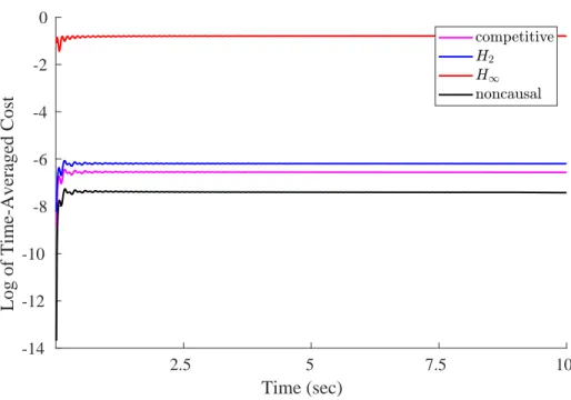
As expected, the optimal path length controller regrets nothing since the path length of the disturbance is zero. We also find that the controller's time-averaged cost 𝐻∞ at steady state approaches 1.00, which is consistent with the fact that its gain 𝐻∞ is 1.00.
Numerical Experiments
Double Integrator
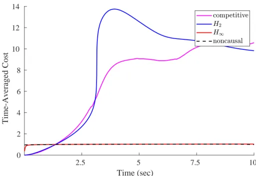
The states of the system are the position and velocity of the object, which are represented by the variables𝑥 ∈Rand𝑥¤ ∈R, respectively. We see that the competitive controller has a lower frequency response than all other causal controllers at all frequencies except near 𝜔 = 0 and 𝜔 = 2𝜋, where the frequency response is highest. The frequency responses in Figure 6.1 predict that the competing controller will perform the best of all the causal controllers; this prediction is confirmed.
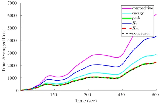
The energy-optimal, path-length-optimal, and 𝐻∞ controllers incur hundreds of times more cost than the competing controller. This huge variation in cost highlights the value of the competitive controller; while it does not always outperform the other causal controllers, it is impossible to engineer perturbations as it incurs hundreds of times more cost than the other controllers.
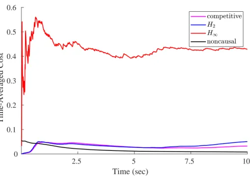
Inverted Pendulum
2 controller will not select the optimal control signal for the nonlinear system due to linearization error. In Figure 6.12, we plot the costs incurred by the causal controllers and the optimal noncausal controller, averaged over ten trials. This is in stark contrast to the 𝐻∞ controller, which incurs hundreds of times more cost than the optimal non-causal controller on some adversarial engineered perturbations.
The 𝐻∞-optimal control problem is to find the controller that minimizes the worst-case gain from the energy in the disturbance𝑤 to the costs incurred by the controller. The 𝐻∞-optimal measurement-feedback control problem is to find the controller that minimizes the worst-case gain from the energy in the disturbances 𝑤and𝑣 at the cost incurred by the controller.
Conclusion and Future Work
Full-Information 𝐻 ∞ control
The finite-horizon 𝐻∞ problem is identical except that the infinite-horizon cost 𝐽(𝜋, 𝑤) is replaced by the finite-horizon cost𝐽𝑇(𝜋, 𝑤). Clearly, if we can solve this suboptimal problem, then we can easily recover the 𝐻∞-optimal controller via halving of𝛾. A strictly causal𝐻∞ controller at level𝛾 exists if and only if conditions (1) and (3) hold, and in addition.
In this case, one possible strictly causal finite-horizon regulator at the 𝛾 level is given by . If the dynamics is time invariant, then this controller converges to the infinite horizon controller described in Theorem 17 as 𝑇.
Measurement-Feedback 𝐻 ∞ control
Clearly, if we can solve this suboptimal problem, then we can easily recover the 𝐻∞-optimal controller by bisection on 𝛾. If these conditions are met, then one possible choice is from 𝑢𝑡 =−𝐾𝑢(b𝑥𝑡+𝑃𝐶∗(𝐼𝑟 +𝐶 𝑃𝐶∗)−1(𝑦𝑡−𝐶 . b𝑥𝑡)), where the state- scoreb𝑥𝑡 is given by recursion. While Theorem 19 tells us how to determine whether there exists a controller 𝐾 such that ∥𝑇𝐾∥ < 1, it does not directly answer the more general question of whether there exists a controller 𝐾 such that ∥𝑇𝐾∥ < 𝛾 for any fixed 𝛾 > 0.
It follows that the controller 𝐾 satisfies ∥𝑇𝐾∥ < 𝛾 in the system 𝐹 , 𝐺 , 𝐻 , 𝐽 is precisely𝛾𝐾b, where𝐾 is the controller satisfying∥𝑇.