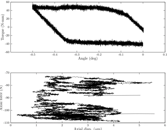
Repeatability of joint-dominated deployable masts

The methods of investigation are experimental measurements of a sample mast and numerical modeling of the mast with special attention to hysteretic joints. Two repetitions of the same bead movement within the same trial are shown.

Figure 1.1: Artist’s depiction of the Shuttle Radar Topography mission above the earth (NASA image [33])

Motivation and goals

More specifically, this thesis will characterize the influence of hysteretic parts and stochastic properties on the linearity and hysteresis of a mast under transient quasi-static loading. The framework for this characterization will be applicable to a variety of mast designs beyond the particular ADAM mast of this study.

Approach

The marriage of detailed characterization of the as-is mast and extensive control over the modeled mast makes it possible to investigate which properties of the mast govern its performance. Analyzing a mast at this level of detail can create a high degree of confidence in its future behavior and focus design and manufacturing efforts on the areas of greatest impact.

Outline

This chapter begins with a literature review that addresses the many studies of lattices, collapsible columns, and joint-dominated structures, including the effects of realistic moving joints and the space environment. Important tools for laboratory and in-flight mast characterization include laser ranging and videogrammetry, and masts of varying degrees of accuracy and stiffness have also been addressed.

Analysis of trusses and deployable masts

In particular, it is noted that the cable must be prestressed to at least the maximum tension of the theoretical part it replaces. Using equivalent stiffness matrices to model the nonlinear behavior of the joint friction, a new iterative matrix model is presented.

Effects of materials and joints

They concluded that "this modeled behavior replicates not only the size of the tumors observed in the experiments, but also the rate of convergence observed in the data." Friction is a leading source of unpredictable behavior in the transition from ground to orbit.

Metrology and experimental methods

Lasers

The metrology system determines the position of the mast tip in three degrees of freedom using a set of two lasers and two position-sensitive detectors. The lasers are attached to the outer tip of the mast and aimed at detectors on the spacecraft's main bus.

Photogrammetry and videogrammetry

By reading the position of the laser dots at a speed above the mast's large natural frequencies, the metrology system will provide decisive data about the pointing of the mast at all times during observation. These corrections will enable the system to achieve a resolution that would otherwise require unusually stable pointing of the 10-m mast.

Other methods

Because the x-ray detectors record the time and impact position of each incoming photon, the reconstructed images can be corrected to account for the motion of the mast tip, even if vibrational modes of the mast are excited during observation. Greschik and Belvin [16] proposed a system of fly beams to support large structures during dynamic testing with minimal disturbance of the vibration mode shapes.

ADAM mast

Applications of ADAM

IPEX-II

This was attributed to “the sudden release of strain energy stored in the hysteretic mechanisms and/or the materials of the structure.” [18, p. Despite this difficulty, the SRTM experiment produced a height map of 80% of the Earth's surface.

Figure 2.11: The SRTM mast (NASA image [33]). The mast is approximately 1 m wide and 60 m long when fully deployed.

Longeron ball-end friction

Experiment

With the longer under pressure, the vertical position of the moving head was fixed and the head was rotated through 0.5◦ and back to its starting position. These were the longons of the four corners of the upper bay of the WSOA mast.

Results

Each corner was tested four times and the stringer rotated to a new position for each of the four tests. Each corner was tested three times and the stringer rotated to a new position for each of the three tests.

Figure 3.3: Force vs. displacment and torque vs. angle curves.

Cable preload

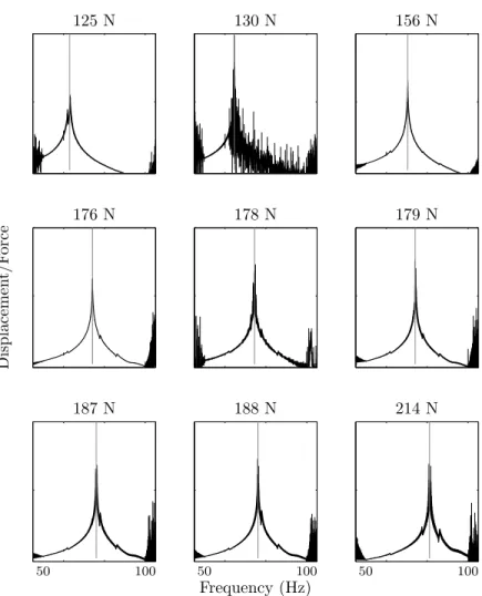
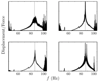
Empirical relationship between tension and vibration frequency

Instead of using the location of the maximum, the resonant frequency was determined by a weighted average. Cable voltage expansion has no clear effect on the resonant frequency of the cable assembly.

Figure 3.8: Mock bay side with inline force sensors.

In situ measurements of cable preload

The mean standard deviation of measurements within a single side was 6 N, while the standard deviation of sixteen mean measurements was 47 N, as illustrated in Figure 3.14. Preload range is an indirect measure of the range of lengths in manufactured parts.

Figure 3.13: Four representative sweeps of Bay 2, Side A. The weighted peak is located at the vertical grey line

Latch and cable behavior

Stiffness of cables
Latch behavior experiment
Analytical model of latch
Results

The purpose of these experiments was to identify a constitutive relationship for the locking of the shape. However, the front surface of the bead and the exact shape of the backstop are both visibly non-ideal, as shown in Figure 3.22.

Figure 3.16: The latching mechanism setup. Two support methods were used without impact on the results: suspension from above and a combination of a hinged support at the weight end with a simple vertical support at the other end.

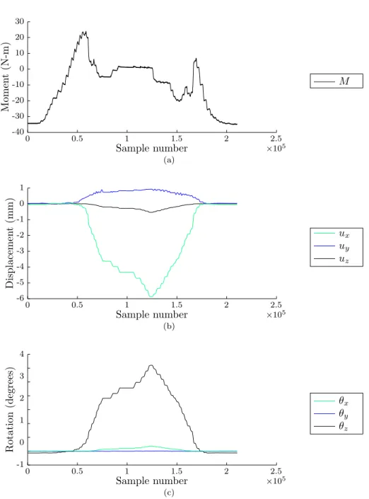
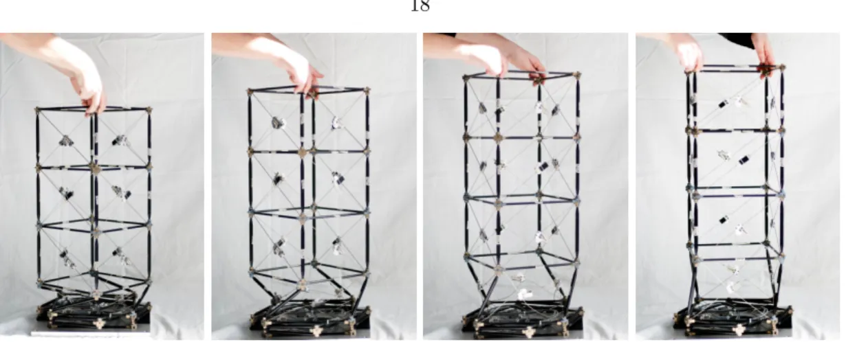
Stowage and deployment

Experiment

At approximately 3◦ rotation, three of the four latches were unlocked and the compartment no longer offered any resistance to further movement. This allowed the weighted cables to apply a deployment torque and return the bay to its original configuration.

Results

Asymmetries in the load and in the behavior of the cargo space components may be a partial reason. This figure shows the path from the node at the center of the top lat square through the displacements ux and uy in the x-y plane.

Figure 4.2: Six degrees of freedom defining the motion of the top batten square.

Shear loading

Experiment

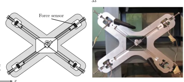
Loads (of magnitude approximately 60 N) were applied in the thex-y plane through a bolt fixed in the center of an aluminum plate, which was attached to the top square joints of the plate. Displacements were measured at the top of the double-bay mast using a beam-finding laser in the same method described in Section 4.1.1.

Results

Therefore, the results for 0◦ and 180◦ should correspond to identical load cases on the mast frame, but they appear to differ, as will be discussed. The orientation of the mast was shifted by 90◦ with respect to its axis between these two data sets.

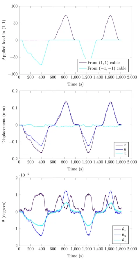
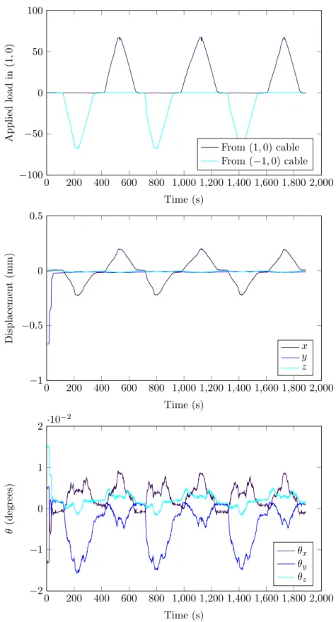
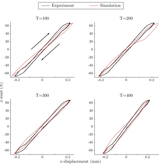
Biaxial shear loading

Experiment

The buckling that appears in the zero-load data is a spurious result that arose from the stiffness assumption of the top square of the panel, which was actually deforming out of square. The tex load cables lie in a plane 57.5 mm above the center of the top square of the panel; their charging cable is 35.5mm above the center of the top square of the panel.

Results

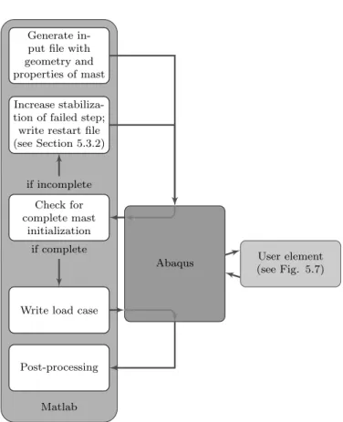
Standard finite elements were used for much of the structure, and are addressed here, and the most essential part of the finite element model is a user element that describes the latch, presented in detail in Section 5.2. The Matlab code, which is fundamental to managing the database of part properties and load cases, will be discussed in Section 5.3.

Figure 4.12: Loading and displacement patterns for the final data set of the biaxial shear experiment.

Basic elements

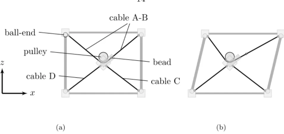
Corner joints and pulleys
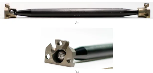
Battens and longerons
Ball-end joints
Cables C and D

The rotation option is used to indicate a relationship between the orientation of the socket node and the longer end. The relationship between the normal load F and the opposite relative rotation moment of the nodes,M, is.

Table 5.1: Properties of modeled battens and longerons.

Latch user element

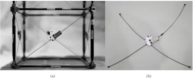
Cable systems

Here the stiffness of the cableEA, the total unstretched lengthL0 and the position of the bead connection in the cable Lb are part of the element properties. This model does not take into account pulley size, non-linear stiffness of the cables or bending stiffness in the cables.

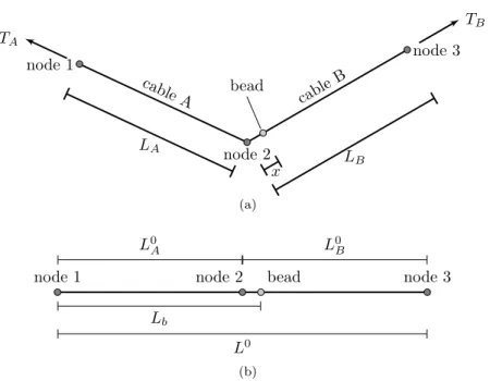
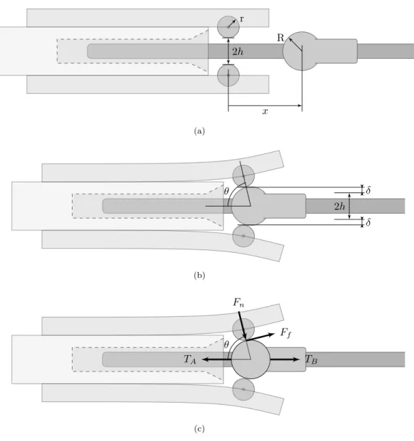
Figure 5.1: Variables for two-section cable. The variables describing the unstretched state are given in (b).

Latch constitutive relationship

It is also convenient to enter the angle between the center line and the line through the center of the bead and the center of a roller, θ(Figure 5.3b) and note that. Now consider the two force components transmitted between the roller and bead: the normal component Fn and the tangential component |Ff| ≤ |µFn| (Figure 5.3c).

Figure 5.3: Geometry of the analytical latch model. The geometry of the unstressed latch, without bead contact, is shown in (a)

Formulation of user element

Because the bead equation ∆T = ∆T(x) is not monotone, it is important to always identify the correct solution of the latch equations. If the solution places x beyond the boundary of the zone, a solution is sought in the next zone in the direction of movement of the bead.

Figure 5.8: An example of the bead zones.

Model generation

Modeling stochastic variability

In this equation, Linitialij is the distance between the two end nodes at the locations where the model is first generated. 100 µm is the face-to-face variability that yields a standard deviation of approximately 50 N in cable tensions.

Initializing the mast model

The position of the masthead is represented by a control node in the center of the upper panel square. Most of the simulation cases apply to the top of the mast a shear load analogous to the experiment of Section 4.2.2.

Figure 5.10: Mast initialization and high-level modeling workflow.

Calibration cases

Batten stiffness

The experiment was originally intended to measure the sliding motion of the entire mast, rather than to measure the stiffness of the batten, and was only later applied to calibrate the modeled stiffness of the batten. This is the reason for the indirect nature of the measurement and the low accuracy of the results.

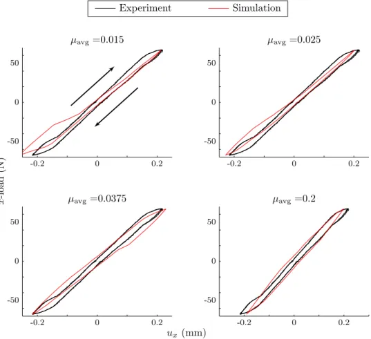
Ball-end friction

A value of µ= 0.0375 is used as the default in the remaining parametric studies, and validation cases are presented for both this value and the experimental mean of µ= 0.14. It is possible that the difference between the range of resting positions of 21µm found experimentally and the 36µm range found at this friction value actually stems from an incorrect value of the friction.

Figure 6.4: Simulation vs. experiment for four values of µ in the longeron ball-end joints.

Impact of modeling practices

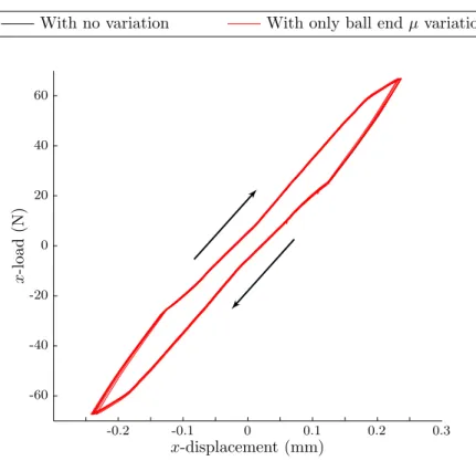
Variability in ball-end friction
Cable preload - variability
Latch model - variability
Measured vs. idealized latch behavior
Geometric imperfections

Selectively removing this variability, as shown in Figure 6.8, shows that this factor does not appear to be the cause of any particular feature in the force-displacement curve. From this we can see that variation in latches is responsible for most of the variation in this measure of behavior, for these levels of variability in each trait.

Figure 6.6: Spread in experimental data with and without variation in the ball-end friction

Component properties

Longeron stiffness

Cable stiffness

The stiffness is considered to be the average of the loading and unloading slopes ∆xload/∆ux. It is quite clear, compared to Figures 6.12 and 6.13, that the shear response is dominated by the cable stiffness rather than the longer stiffness.

Mean cable preload

The four corner joints of the base were fully constrained in all size degrees of freedom with the *BOUNDARY command. In all cases, the simulation load or displacement condition was applied to the control node.

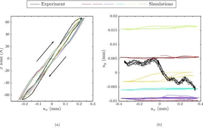
Figure 6.14: Simulation vs. experiment for four values of preload tension in the cables.

Torsional motion

Three models generated with independent stochastic component properties are included in (a), while a single model is run through multiple rotation loops in (b). Four models generated with independent stochastic component properties are included in (a), while a single model is run through multiple rotation loops in (b).

Figure 7.1: Twist vs. moment for the experiment and simulation with the calibrated ball-end friction value

Shear loading

The most significant point of agreement between experiment and model is that the displacement curve shows none of the distortions associated with decoupling. In this load case, the model correctly predicts that the beads rest against the abutments and do not produce the characteristic broadening of the force-displacement curve seen when the closures begin to detach.

Biaxial shear loading

The behavior of the mast was mainly characterized by the resting range of the unloaded mast after transient quasi-static shear loading. The initial position of the face corresponding to the zero reading of the laser is known.

Figure 7.6: Shear in the x direction with zero y load for six two-bay mast models with stochastic component behaviors

Mast generation pseudocode

At this point, there is a comprehensive solution to the current state of the latch and cable. C The reaction force is the magnitude of the tension in the C direction of the cable.