Response Time - Mode 1 History for a 6-story Controlled Primary Category 1 System Subjected to (a) EI Centro, (b) Taft Lincoln School Tunnel, and (c) Holiday Inn Excitation Records. Response Time - Mode 2 History for a Category 2 6-story Supervised Primary System Subjected to (a) EI Centro, (b) Taft Lincoln School Tunnel, and (c) Holiday Inn Excitation Records.
List of Tables
Peak and Root Mean Square Values of Nodal Mass Acceleration (Absolute) for a 6-Storey Controlled Primary Category 3(b) System Using Type 1 Elements Peak and Root Mean Square Values of Nodal Mass Acceleration (Absolute) for a 3-Storey Controlled Primary Category 3 System (b) which uses type 1 elements.
Introduction and Background
Introduction
Background
Instead, the normal force merely changes the mechanical properties of the device (i.e., the slip force level) responsible for the interactions between the structures. The operation of the bracket was controlled by varying the clamping force on the friction surface of the slip device to control the reaction force transmitted to the structure.
Description and Organization of the Thesis
In Chapter 3, a preliminary study of the proposed control approach is performed within the specialized setting of linear single-degree-of-freedom (SDOF) primary and auxiliary systems. The effectiveness of the control approach is assessed by comparing the response of the controlled primary system with that of an uncontrolled primary system.
Kamagata, "A proposal of new anti-seismic structure with active seismic response control system - dynamic intelligent system," Paper SE-ll, Proc. Ishii, “Seismic Response Controlled Structure with Active Mass Manager System and Active Variable Stiffness System,” Proc.
Classical, Instantaneous, and Incremental Optimal Control Methods
Introduction
Definition and Formulation of an Optimal Control Process
In fact, one of the tasks involved in the synthesis of an optimal control process is to determine each of these objects if there is some freedom in their choice. For each control process U, a real scalar quantity J[U], known as a performance index, can be assigned by a relation of the form.
Necessary Conditions for an Optimal Control Process
The admissible control input functions considered herein are assumed to be at least piecewise continuous. In cases for which the control input vector is constrained to belong to some specified set of admissible functions; U E n, with n c Rr; the minimum principle of Pontryagin [5] is used (see Appendix A).
Classical Optimal Control Methods
The special case of interest is that for which Zb is free but tb is fixed, and. To obtain a relation that can be used to find this form, (2-20) is differentiated to give 2-24) Since the relation in (2-24) must hold at every z along the optimal path for any given za' it is necessary to.
Instantaneous Optimal Control Methods
In view of the previous results, the following approach is proposed for the control of linear dynamic systems subjected to external excitations for which no prior information is available. When u and v are nonzero, the effect of the control strategy is to immediately minimize the integrand of the first integral in (2-77), which represents the accumulation rate of J contributed by the control input.
Incremental Optimal Control Methods
The amplified system controlled by the dynamic equation in (2-102) and the performance index as expressed in (2-103) is now in a form suitable for application of the incremental optimal control method outlined above . 2-107) Thus, the specifications for the operation of the dynamic controller according to the incremental optimal control method are complete.
Summary
Response Control of Linear SDOF Systems Using Active Interface Damping
Introduction
In the present study, the control effort is aimed at reducing the relative displacements caused by the excitation. The stresses induced in the structure are directly proportional to these displacements when deformations are within the linear-elastic range of the material of which the structure is composed.
Problem Formulation
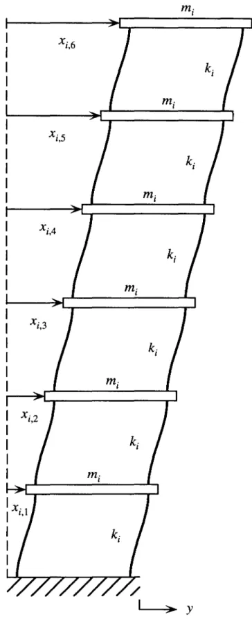
The scalar pair (x;, x;), which consists of the vector Zi', is called the state of the ith dynamic system. The state of a dynamic system is an embodiment of the minimum amount of information at a given moment of time, which, together with the equation governing the dynamic behavior of the system, is sufficient to determine the state of the system at all future points of time. . Loosely speaking, the state of a system consists of a certain set of defining conditions associated with that system.
Control Strategy
These mechanical properties dictate the physical nature of the interactions and consequently the control input values used for the sampling period. For each of these methods, let 11 (t) be the functional form for 11' the value of the control force applied by the interacting element to the primary system. In addition, the quantities that multiply h in the second term of (3-12) are fixed regardless of the operating condition chosen for the interacting element.
Interaction Elements
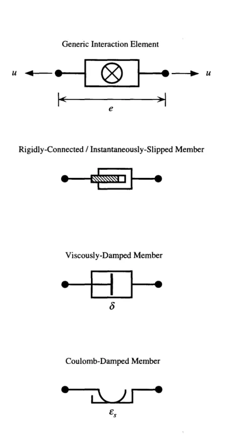
To facilitate the implementation of the control strategy by the two methods discussed in the previous section, several interaction elements are considered. For the control cases using Method 1, three types of interaction items are used separately to examine the effectiveness of the control approach. It is not necessary to specify the precise physical nature of the interaction element for the control cases using method 2, since the activation-deactivation process is modeled to occur instantaneously.
Numerical Study
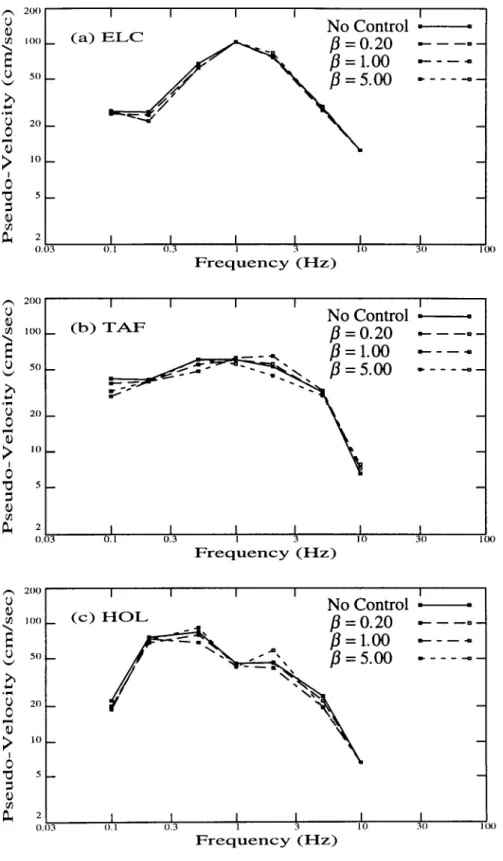
This ensemble consists of the 1940 Imperial Valley (EI Centro) SOOE, 1952 Kern County (Taft Lincoln School Tunnel) S69E, and 1971 San Fernando (Holiday Inn) NOOW earthquake records. In turn, the dynamic behavior of the auxiliary system is fully characterized by specifying the dimensionless parameters. The connection created is then immediately terminated, allowing the systems to move independently for the duration of the sampling period.
Control Algorithms
At the beginning of each sampling period, the conditions of the primary and auxiliary systems are measured or evaluated. The control processor then estimates the rate at which relative vibrational energy is added to the primary system as a result of the interaction (given by the term multiplying h in (3-12). Also, for cases in categories 2 and 3, the onset of an interaction is allowed only when both the conditions of the basic criterion and those of the additional criterion related to the connection process are met.
Results
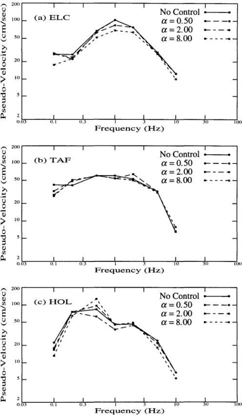
The spectra for all cases are shown in Figure 3.7 for each of the excitation records. The spectra for all cases are shown in Figure 3.8 for each of the excitation records. The response spectra for the controlled cases are generally reduced compared to the response spectrum for the uncontrolled case for each of the excitation records considered.
Discussion
The response spectra for the controlled cases in this category, which is included in the study mainly for comparison purposes with Category 9, are shown in Figures 3.24 to 3.28 for each of the excitation records. Thus, for the purposes of this study, this control algorithm will be referred to as the Kajima A VS control algorithm. It is clear that more energy is dissipated per cycle for the case using the proposed control algorithm than .
Response spectra of category 1 controlled cases for various values of a - with f3 = 0 and r = 0 - for (a) El Centro, (b) Taft Lincoln School Tunnel, and (c) Holiday excitation recordings Inn. Response spectra of category 1 controlled cases for various values of a - with f3 = 0 and r = 0 - for (a) EI Centro, (b) Taft Lincoln School Tunnel, and (c) Holiday excitation recordings Inn. Response spectra of category 3 controlled cases for various values of a - with f3 = 0.20 and r = ~ af3 - for (a) El Centro, (b) Taft Lincoln School Tunnel, and (c) Records of Holiday Inn harassment.
Response spectra of category 4 controlled cases for various values of /3 - with a = 0 and r = 0 - for (a) EI Centro, (b) Taft Lincoln School Tunnel, and (c) Holiday Inn Excitation Records. Response spectra of category 5 controlled cases for various values of a - with f3 = 0.20 and r = ,j af3 - for (a) EI Centro, (b) Taft Lincoln School Tunnel, and (c) Holiday Inn Excitation Records.
Response Control of Linear MDOF Systems Using Active Interface Damping
Introduction
Problem Formulation
U E R', referred to as the control input, represents the reaction forces developed within each of the interacting elements. Because each of the interacting elements is treated as massless, a relationship exists between the control force acting on the ith system and the control input, given by . From (4-12) it is clear that the equations represented in (4-9), which govern the ni reaction modes of the i-th system, can be represented equivalently by a set of ni decoupled equations, where the jth equation is given by.
Control Strategy
In fact, attention will be focused on the relative vibrational energy present in the dominant response mode of the primary system. The contribution of the control input to the response mode j of the ith system depends on both the prescribed values of Uk and the entries of column j of p;u. If possible, the values of Uk should be chosen to achieve a desirable control effect for the ith system.
Interaction Elements
According to the previous discussion, it is convenient to solve (4-34), representing Maxwell's viscoelastic element, for the reactive force in terms of the strain history of the element (to avoid confusion in notation, let £ denote the strain of the element , and let e(·) denote the scalar exponential function). For cases where a Type 1 element is used, deactivating the element instantly creates a zero value for reaction force (this value lasts as long as the element is deactivated), while a new level of reaction force is not created immediately when the element is activated. A type 1 element can be considered a special case of a type 2 element in which either
Numerical Study
As is done for the cases in category 3(b), all the cases in this category assume that the auxiliary system is much stronger and more massive than the primary system. A single interaction element is attached between this small mass and the roof plate of the primary system, as illustrated in Figure 4.6. Because of these properties, the relative displacements of the auxiliary system are not directly affected by the base acceleration.
Control Algorithms
Then, because the operating state of each element can be selected independently of the other elements, the following conditions are used to determine. A two-step procedure is then used to select the appropriate operating state for each of the elements. Since dynamic elements are used, the values for each of the UK are fixed at a.
Results
Finally, Figure 4.22 shows the response of Mode 1 for a case that corresponds to the control case used for Figure 4.16, but for which only the top three elements participate. Finally, Figure 4.29 shows the response of Mode 1 for a case corresponding to the control case used for Figure 4.23, involving a 6-6 primary-auxiliary system configuration in which only the top three elements participate. Finally, Figure 4.36 shows the response of Mode 1 for a case corresponding to the control case used for Figure 4.30, involving a 6-6 primary-auxiliary configuration in which only the top three elements participate.
Discussion
Significant response reduction is achieved in the first mode for each of the excitation records. Figures 4.54 and 4.55 show the results of the reaction control effort for cases in which: only. Now consider a situation in which all the elements are simultaneously either enabled or disabled.
Mode 1, (b) Mode 2, and (c) Mode 3 for a 6-story uncontrolled primary system subjected to the El Centro excitation record. (a) Mode 1, (b) Mode 2, and (c) Mode 3 response time histories for a 6-story uncontrolled primary system subjected to the Holiday Inn Excitation Record. (a) Mode 1, (b) Mode 2, and (c) Mode 3 response time histories for a 3-story uncontrolled primary system subject to the Holiday Inn Excitation Record.